Tricks with match bonus or how to fool Dijkstra’s limitations Link to heading
The reader is assumed to have basic knowledge about pairwise alignment and graph theory.
In this post we will show how to transform traditional alignment score models that include a match bonus into an equivalent cost model using only non-negative costs. We generalize the relationship in Eizenga and Paten (2022) and show that it applies to both affine and asymmetric cost models. Unlike their method, our method does not increase the base penalties by a factor \(2\), leading to a lower cost alignment, and hence a potentially faster runtime of WFA.
Tl;dr: Negative match costs can be transformed into an equivalent non-negative cost model. This allows WFA to solve such instances of global alignment, and may provide up to 2x speedup over an earlier transformation.
Edit graph Link to heading

Figure 1: The edit graph with match cost (M=0), mismatch cost (X), insertion cost (I), and deletion cost (D).
The default global pairwise alignment task can be considered as the task of finding a shortest path in the edit graph, as shown in Figure 1.
Edges in this graph correspond to the cost you need to ‘pay’ for an insertion (cost \(I\)), deletion (cost \(D\)), or mismatch (cost \(X\)) of a letter. If two letters are the same, you can go through a ‘match’ edge for free (cost \(M=0\)). Since matches are free, it is allowed to greedily match characters whenever possible without considering the insertion and deletion edges. This principle is the basis of the WFA algorithm, which can extend diagonals efficiently because it does not check other operations.

Figure 2: Edit graph with negative match cost (M=-B).
In some cases, a negative match cost \(M<0\) is used, where using a match decreases the cost of the alignment, as in Figure 2. We call the positive number \(B:=-M\) the match bonus.
Algorithms Link to heading
Let’s briefly recall what algorithms can be used to compute the shortest path in an edit graph. (Note: \(n\) and \(m\) are sequence lengths here, and \(s\) is the distance between them.)
- Needleman-Wunsch: \(O(nm)\) approach based on dynamic programming that works for any cost model.
- Exponential band: \(O(ns)\) by doubling the searched band on each iteration. Only for non-negative costs.
- Dijkstra: \(O(ns)\) when used with a bucket-queue. Only works for non-negative costs.
- WFA: A more efficient variant of Dijkstra, \(O(ns)\) worst case and \(O(s^2)\) expected case. Only works for non-negative edges.
As you can see, only the Needleman-Wunsch DP can handle the negative cost edges created by introducing a match bonus.1 All other algorithms break.
Potentials Link to heading
A classic variant of Dijkstra’s algorithm that can handle negative-cost edges is Johnson’s algorithm (Johnson 1977). The idea is to give a potential \(\phi(u)\) to each vertex \(u\), and change the cost of an edge from \(u\) to \(v\) from \(E(u, v)\) to2 \[E’(u,v) = E(u,v) - \phi(u) + \phi(v).\] Regardless of how the potential function \(\phi\) is chosen, the length of each path from any vertex \(s\) to any vertex \(t\) will change by exactly \(\phi(t) - \phi(s)\). This means that the transformation preserves shortest paths.
It turns out \(\phi\) can always be chosen in such a way that all new edge costs \(E’\) are non-negative when the graph does not contain negative cycles. In particular, in Jonson’s algorithm \(-\phi(u) = d(s, u)\) is the length of the shortest path from a fixed vertex \(s\) to \(u\). This somewhat defeats our purpose though: computing shortest paths is what we are trying to do in the first place.
In our case, the edit graph is weighted, directed, without cycles, and “all roads lead to Rome” in it – any way you can take in the edit graph will end in the target point to which we are finding a shortest path. To get to this terminus we need to cross the graph both vertically and horizontally as we go from the upper left corner to the bottom right one. All paths take the same number of steps down, and the same number of steps to the right, where an insertion is one step down, a deletion is one step right, and a match and mismatch are counted as one step down and one step right.

Figure 3: Edit graph with transformed non-negative edges with (Delta_D + Delta_I = B), so that (M’=0).
We can increase the cost of each horizontal step by \(\Delta_D\) and the cost of each vertical step by \(\Delta_I\) (Figure 3), so that (mis)matches become \(\Delta_I+\Delta_D\) more expensive. This way, the total cost of the alignment goes up by \(n\cdot \Delta_D + m \cdot \Delta_I\).
Now, a simple way to get rid of negative match edges is to simply require that \(\Delta_I + \Delta_D \geq B\).

Figure 4: Coordinate grid for states/vertices.
Let \(u=\langle i, j\rangle\) denote the vertex in column \(i\) and row \(j\) (Figure 4). Then, the above is equivalent to a potential \(\phi\) given by \[\phi(u) = \phi\langle i, j\rangle := i\cdot \Delta_D + j\cdot \Delta_I.\]
Indeed, the cost of a deletion goes up by \(\Delta_D\) \[D’ := D - \phi\langle i, j\rangle + \phi\langle i+1, j\rangle = D + \Delta_D,\] and the cost of an insertion edge goes up by \(\Delta_I\): \[I’ := I - \phi\langle i, j\rangle + \phi\langle i, j+1\rangle = I + \Delta_I.\] Similarly, for matches and mismatches, the cost goes up by \(\Delta_I + \Delta_D\),
\begin{align} X’ &:= X + \Delta_D + \Delta_I,\\ M’ &:= M + \Delta_D + \Delta_I. \end{align}
We would like all edges to have a non-negative cost, so our choice of \(\Delta_D\) and \(\Delta_I\) must satisfy the following constraints:
\begin{align} \Delta_D &\geq -D,\\ \Delta_I &\geq -I,\\ \Delta_D + \Delta_I &\geq -M = B \geq 0. \end{align}
Multiple variants Link to heading
The above equations give us some flexibility in choosing \(\Delta_I\) and \(\Delta_D\). We will restrict ourselves to the case where \(M’ = M + \Delta_D + \Delta_I = 0\), i.e. where exact matches are free.
There are a few natural choices of \(\Delta_D\) and \(\Delta_I\) that we cover in the table below.
| Type | \(\Delta_D\) | \(\Delta_I\) | \(M’\) | \(X’\) | \(D’\) | \(I’\) |
|---|---|---|---|---|---|---|
| Symmetric | \(\lfloor B/2 \rfloor\) | \(\lceil B/2\rceil\) | \(0\) | \(X+B\) | \(D+\lfloor B/2\rfloor\) | \(I+\lceil B/2\rceil\) |
| Expensive deletions | \(B\) | \(0\) | \(0\) | \(X+B\) | \(D+B\) | \(I\) |
| Expensive insertions | \(0\) | \(B\) | \(0\) | \(X+B\) | \(D\) | \(I+B\) |
| Free deletions | \(-D\) | \(B+D\) | \(0\) | \(X+B\) | \(0\) | \(I+B+D\) |
| Free insertions | \(B+I\) | \(-I\) | \(0\) | \(X+B\) | \(D+B+I\) | \(0\) |
The symmetric option in the first row is the most natural choice, and roughly corresponds to the transformation suggested in Eizenga and Paten (2022). It differs in that all costs are divided by \(2\) and the half-integer costs in the odd \(B\) case are distributed between \(I’\) and \(D’\).
The bottom two rows are even applicable when matches are already free (\(B=0\)), and transfer the cost of horizontal steps to vertical steps or vice-versa by increasing \(D\) and decreasing \(I\) by the same amount.
Some notes on algorithms Link to heading
WFA Link to heading
For WFA this cost transformation is a life-saver because with \(M’=0\) it allows for “greedy matching” again—the core of the algorithm that enables fast extending diagonals. This is important, because one of the main WFA data structures is a wavefront, which covers all states that can be reached with specific cost. If the cost could go down, it could disrupt previous wavefronts, which would break the logic of the algorithm. The drawback of the cost transformation is that it increases the cost of the optimal alignment, and hence increases the number of wavefronts, leading to a slower WFA execution.
Thus, we expect that the lower the potential of the target state, the faster the WFA algorithm runs.
A* Link to heading
The A* algorithm by itself can not handle negative costs. However, a heuristic function \(h\) can be modified to achieve exactly the same result as the potentials introduced above by using
\begin{equation} h’(u) := h(u) + \phi(u). \end{equation}
This works in our case because it ensures that \(f(u) = g(u) + h’(u)\) can never decrease when taking an edge.
Extending to different cost models Link to heading
Affine costs Link to heading
The potentials defined above naturally extend to affine costs. Each state in an affine layer naturally corresponds to a state \(\langle i,j\rangle\) in the main layer, and can use the corresponding potential.
This means that the delete-extend cost increases with \(\Delta_D\), and similarly the insert-extend cost increases with \(\Delta_I\), while gap-open costs remain the same.
Substitution matrices Link to heading
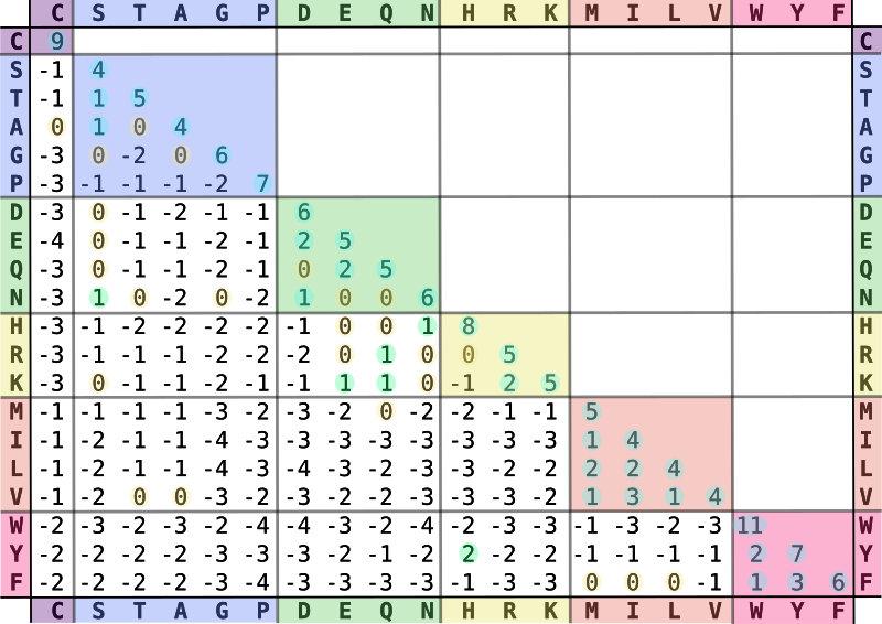
Figure 5: The BLOSUM matrix. CC BY-SA 4.0 via Wikipedia.
The BLOSUM matrix (Figure 5) specifies a match score for each pair of amino acids, with some entries being positive (indicating similarity) and some being negative, so we are maximizing the score. This can be transformed into a cost model by simply negating all scores, which allows us the previous techniques.
In general, let \(B\) be the maximum score assigned to any pair of letters in the substitution matrix \(S\),3 i.e. the maximum entry in the matrix. Again we choose \(\Delta_D\) and \(\Delta_I\) such that \(\Delta_D + \Delta_I \geq B\). Then, we simply replace each matrix element \(S_{xy}\) by \(S_{xy}’ = S_{xy} - \Delta_D - \Delta_I\), ensuring that all the scores are at most \(0\).
But not local alignment Link to heading
We will stress here that this idea does not work for local alignment. The reason it works for global alignment is that the cost of each path is increased by the same amount. Two local alignments can have completely different lengths and thus span a different number of rows/columns of the table. That means that the cost increase \(\phi(end) - \phi(start)\) of these two local alignments is different, and hence their final scores are not directly comparable.
Evaluations Link to heading
Now let’s see how WFA performs when using different transformation variants.
We will use the following cost model:
- \(I = 1\) - insertion cost
- \(D = 1\) - deletion cost
- \(X = 1\) - substitution cost
- \(B = 2\) - match bonus
Unequal string length Link to heading
Firstly, let’s make an experiment on sequences where the first sequence is longer than the second, i.e. \(|A| = n > m = |B|\).
Given the match bonus, we can take different values for \(\Delta_I\) and \(\Delta_D\). According to our hypothesis of keeping the cost increase minimal, the optimal option should be \(\Delta_I = 2\) and \(\Delta_D = 0\), since \(\Delta_I\) is multiplied by \(m=\min(m,n)\). Let’s check that!4, 5
[TODO: Also compare to the transformation in Eizenga and Paten (2022).]
| \(n\) | \(m\) | \(\Delta_D\) | \(\Delta_I\) | Cost | Time (ms) | #expanded |
|---|---|---|---|---|---|---|
| 260 | 199 | \(2\) | \(0\) | -275 | 26 | 92628 |
| 260 | 199 | \(1\) | \(1\) | -275 | 11 | 48895 |
| 260 | 199 | \(0\) | \(2\) | -275 | 6 | 42610 |
| 260 | 199 | \(D + b\) | \(I + b\) | -275 | 26 | 97477 |
Note: the last row in the table depictes experiment on cost model with match bonus introduced in Eizenga and Paten (2022), so \(\Delta_D + \Delta_I\) is not required to be equal to \(b\) in this particular case.
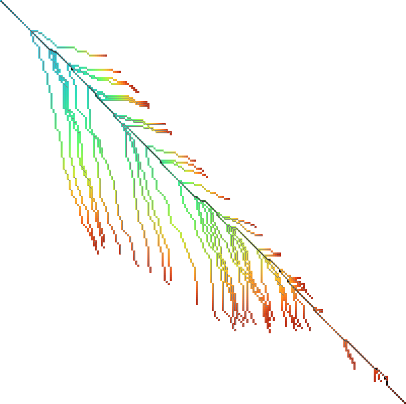
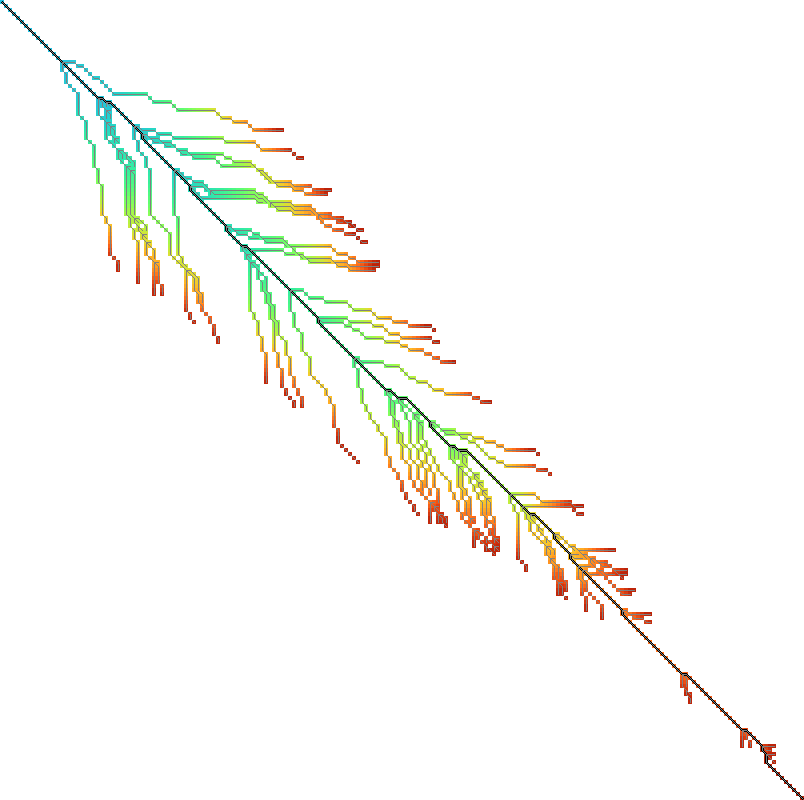
The numbers are eloquent enough, so let’s look at the pixels. As you can see the second sequence has a suffix of the first one deleted.
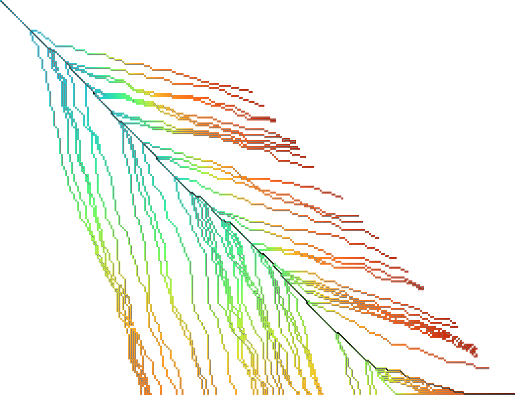 |  |  |
We can clearly see that increasing \(\Delta_I\) (the vertical cost) instead of \(\Delta_D\) (the horizontal cost) yields less downward expansion, and fewer visited states in total.
Equal string lengths Link to heading
Let’s see how things work out in case of equal length strings, where the total score will be the same independent of how we choose \(\Delta_D\) and \(\Delta_I\).
| N | M | \(\Delta_D\) | \(\Delta_I\) | Cost | Time (ms) | #expanded |
|---|---|---|---|---|---|---|
| 200 | 200 | \(2\) | \(0\) | -323 | 4 | 45920 |
| 200 | 200 | \(1\) | \(1\) | -323 | 3 | 34466 |
| 200 | 200 | \(0\) | \(2\) | -323 | 4 | 46020 |
| 200 | 200 | \(D + b\) | \(I + b\) | -323 | 6 | 68669 |
Note: the last row in the table depictes experiment on cost model with match bonus introduced in Eizenga and Paten (2022), so \(\Delta_D + \Delta_I\) is not required to be equal to \(b\) in this particular case.
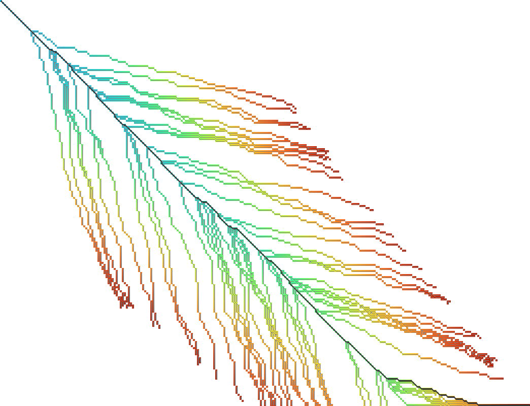
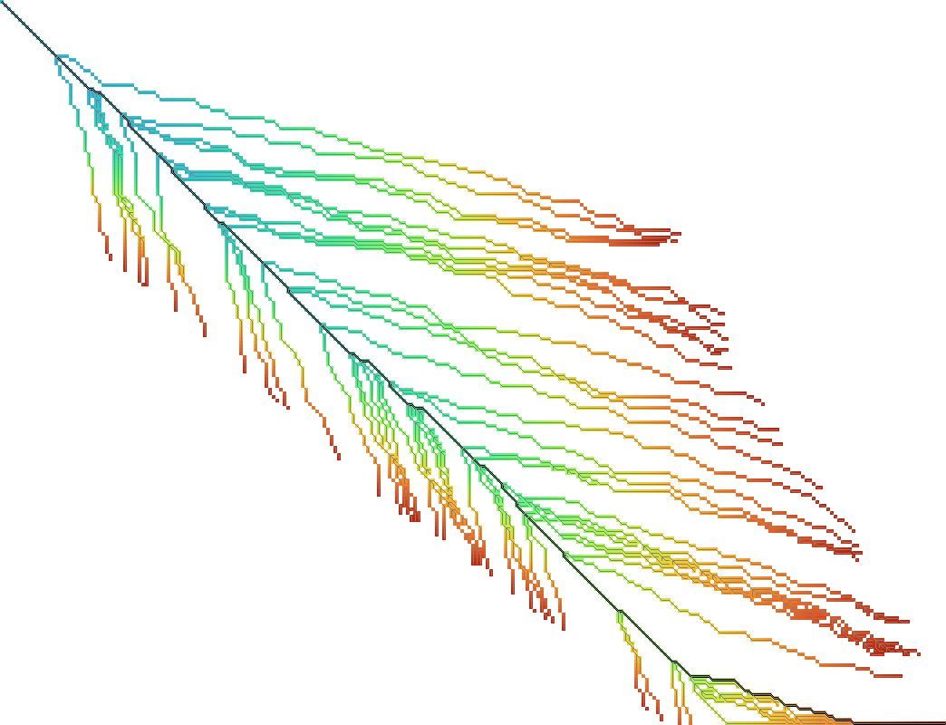
In this case, we can see in the experiments that it is preferred to split the match bonus equally between \(\Delta_D\) and \(\Delta_I\). Pictures for this case are so:
 |  | 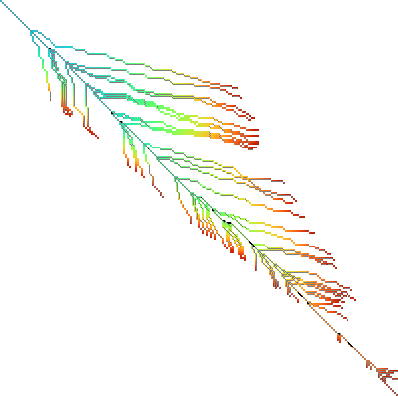 |
The middle picture clearly visits fewer states, and seems to benefit from being pushed towards the end, without needless exploration to the sides.
Conclusion Link to heading
We have shown that alignment score/cost models that include a match bonus can be transformed into an equivalent cost model using only non-negative costs when doing global alignment. This transformation even works for affine and asymmetric costs. It avoids doubling costs (to preserve integral values) by distributing an odd match bonus unevenly over the horizontal and vertical steps in the edit graph.
To summarize: when the cost model is given by match cost \(M=-B\), mismatch cost \(X\), insertion cost \(I\), and deletion cost \(D\), the equivalent cost model for global alignment with non-negative costs is given by:
\begin{align} M’ &= 0,\\ X’ &= X+B,\\ D’ &= D + \lfloor B/2 \rfloor,\\ I’ &= I + \lceil B/2 \rceil. \end{align}
References Link to heading
That’s because NW visits all vertices in topologically sorted order, and hence considers all possible path to each vertex. ↩︎
Note that most sources use \(\phi\) with an opposite sign. We find our choice to be more natural though: think of the potential as potential energy (height). When going up, you pay extra for this, and can use this energy/cost reduction later when going down. ↩︎
I’m using \(S\) instead of \(M\) to indicate that this is a score instead of a cost. ↩︎
The author’s laptop was made in times of the Second Punic War, so he decided not to take very long sequences to save his working station. ↩︎
Also, the code is not optimized in the first place. Look at relative timings only. ↩︎