- Abstract
- 1 Introduction
- 1.1 Contributions
- 1.2 Previous work
- 1.2.1 Needleman-Wunsch
- 1.2.2 Graph algorithms
- 1.2.3 Computational volumes
- 1.2.4 Parallelism
- 1.2.5 Tools
- 2 Preliminaries
- 3 Methods
- 3.1 Band-doubling
- 3.2 Blocks
- 3.3 Memory
- 3.4 SIMD
- 3.5 SIMD-friendly sequence profile
- 3.6 Traceback
- 3.7 A*
- 3.7.1 Bulk-contours update
- 3.7.2 Pre-pruning
- 3.8 Determining the rows to compute
- 3.9 Incremental doubling
- 4 Results
- 5 Discussion
- Acknowledgements
- Conflict of interest
- 6 Appendix
\begin{equation*} \newcommand{\g}{g^*} \newcommand{\h}{h^*} \newcommand{\f}{f^*} \newcommand{\cgap}{c_{\textrm{gap}}} \newcommand{\xor}{\ \mathrm{xor}\ } \newcommand{\and}{\ \mathrm{and}\ } \newcommand{\st}[2]{\langle #1, #2\rangle} \newcommand{\matches}{\mathcal M} \end{equation*}
This post was published at WABI24 (PDF). Content below is slightly out of sync.
Groot Koerkamp, Ragnar. 2024. “A*PA2: Up to 19 Faster Exact Global Alignment.” In Wabi 2024, 312:17:1–17:25. Lipics. https://doi.org/10.4230/LIPIcs.WABI.2024.17.
Abstract Link to heading
Methods. We introduce A*PA2, an exact global pairwise aligner with respect to edit distance. The goal of A*PA2 is to unify the near-linear runtime of A*PA on similar sequences with the efficiency of dynamic programming (DP) based methods. Like Edlib, A*PA2 uses Ukkonen’s band doubling in combination with Myers’ bitpacking. A*PA2 1) extends this with SIMD (single instruction, multiple data), 2) uses large block sizes inspired by Block Aligner, 3) avoids recomputation of states where possible as suggested before by Fickett, 4) introduces a new optimistic technique for traceback based on diagonal transition, and 5) applies the heuristics developed in A*PA and improves them using pre-pruning.
Results. The average runtime of A*PA2 is \(19\times\) faster than BiWFA and Edlib on $>500$kbp long ONT reads of a human genome having \(6\%\) divergence on average. On shorter ONT reads of \(11\%\) average divergence the speedup is \(5.6\times\) (avg. length $11$kbp) and \(0.81\times\) (avg. length $800$bp).
Availability. https://github.com/RagnarGrootKoerkamp/astar-pairwise-aligner
Contact. https://twitter.com/curious_coding
1 Introduction Link to heading
The problem of global pairwise alignment is to find the shortest sequence of edit operations (insertions, deletions, substitutions) to convert a string into a second string (Needleman and Wunsch 1970; Vintsyuk 1968), where the number of such operations is called the Levenshtein distance or edit distance (Levenshtein 1965; Wagner and Fischer 1974).
Over time, the length of genomic reads has increased from hundreds of basepairs to hundreds of thousands basepairs now. Meanwhile, the complexity of exact algorithms has not been improved by more than a constant factor since the introduction of the diagonal transition algorithm (Ukkonen 1985; Myers 1986).
Our recent work A*PA (Groot Koerkamp and Ivanov 2024) uses the A* shortest path algorithm to speed up alignment and has near-linear runtime when divergence is low. A drawback of A* is that it uses a queue and must store all computed distances, causing large overhead compared to methods based on dynamic programming (DP).
This work introduces A*PA2, a method that unifies the heuristics and near-linear runtime of A*PA with the efficiency of DP based methods.
As Fickett (1984, 1) stated 40 years ago and still true today,
at present one must choose between an algorithm which gives the best alignment but is expensive, and an algorithm which is fast but may not give the best alignment.
In this paper we narrow this gap and show that A*PA2 is nearly as fast as approximate methods.
1.1 Contributions Link to heading
We introduce A*PA2, an exactly pairwise global sequence aligner with respect to edit distance.
In A*PA2 we combine multiple existing techniques and introduce a number of new ideas to obtain up to \(19\times\) speedup over existing single-threaded exact aligners. Furthermore, A*PA2 is often faster and never much slower than approximate methods.
As a starting point, we take the band doubling algorithm implemented by Edlib (Šošić and Šikić 2017) using bitpacking (Myers 1999). First, we speed up the implementation (points 1., 2., and 3.). Then, we reduce the amount of work done (points 4. and 5.). Lastly, we apply A* (point 6.).
- Block-based computation. Edlib computes one column of the DP matrix at a time, and for each column decides which range (subset of rows) of states to compute. We significantly reduce this overhead by processing blocks of \(256\) columns at a time (Table 1f), taking inspiration from Block aligner (Liu and Steinegger 2023). Correspondingly, we only store states of the DP-matrix at block boundaries, reducing memory usage.
- SIMD. We speed up the implementation using $256$bit SIMD to compute each block, allowing the processing of \(4\) computer words in parallel.
- Novel encoding. We introduce a novel encoding of the input sequence to
speed up SIMD operations by comparing characters bit-by-bit and avoiding slow
gatherinstructions. This limits the current implementation to size-\(4\) alphabets. - Incremental doubling. Both the band doubling methods of Ukkonen (1985) and Edlib recompute states after doubling the threshold. We avoid this by using the theory behind the A* algorithm, extending the incremental doubling of Fickett (1984) to blocks and arbitrary heuristics.
- Traceback. For the traceback, we optimistically use the diagonal transition method (Ukkonen 1985; Myers 1986; Marco-Sola et al. 2021) within each block with a strong adaptive heuristic, falling back to a full recomputation of the block when needed.
- A* . We apply the gap-chaining seed heuristic of A*PA (Groot Koerkamp and Ivanov 2024) (Table 1fg), and improve it using pre-pruning. This technique discards most of the spurious (off-path) matches ahead of time.
 |  |  |  |  |  | |
|---|---|---|---|---|---|---|
| + DT | + band doubling | + gap heuristic and bitpacking | + blocks | + GCSH | A* | |
| Dijkstra | WFA | Ukkonen | Edlib | A*PA2-simple | A*PA2-full | A*PA |
1.2 Previous work Link to heading
In the following, we give a brief recap of developments that this work builds on, in chronological order per approach. See also e.g. the reviews by Kruskal (1983) and Navarro (2001), and the introduction of our previous paper Groot Koerkamp and Ivanov (2024). 2 covers relevant topics more formally.
1.2.1 Needleman-Wunsch Link to heading
Pairwise alignment has classically been approached as a dynamic programming problem. For input strings of lengths \(n\) and \(m\), this method creates a \((n+1)\times (m+1)\) table that is filled cell by cell using a recursive formula. Needleman and Wunsch (1970) gave the first \(O(n^2m)\) algorithm, and Sellers (1974) and Wagner and Fischer (1974) improved this to what is now known as the \(O(nm)\) Needleman-Wunsch algorithm, building on the quadratic algorithm for longest common subsequence by Sankoff (1972).
1.2.2 Graph algorithms Link to heading
It was already realized early on that an optimal alignment corresponds to a shortest path in the edit graph (Vintsyuk 1968; Ukkonen 1985) (see 2). Both Ukkonen (1985) and Myers (1986) remarked that this can be solved using Dijkstra’s algorithm (Dijkstra 1959), taking \(O(ns)\) time (Table 1a), where \(s\) is the edit distance between the two strings and is typically much smaller than the string length. (Although Ukkonen only gave a bound of \(O(nm \log (nm))\).) However, Myers (1986, 2) observes that
the resulting algorithm involves a relatively complex discrete priority queue and this queue may contain as many as \(O(ns)\) entries even in the case where just the length of the […] shortest edit script is being computed.
Hadlock (1988) realized that Dijkstra’s algorithm can be improved upon by using A* (Hart, Nilsson, and Raphael 1968), a more informed algorithm that uses a heuristic function \(h\) that gives a lower bound on the remaining edit distance between two suffixes. He uses two heuristics, the widely used gap cost heuristic (Ukkonen 1985; Hadlock 1988; Wu et al. 1990; Spouge 1989, 1991; Papamichail and Papamichail 2009) that simply uses the difference between the lengths of the suffixes as lower bound (Table 1d), and a new improved heuristic based on character frequencies in the two suffixes. A*PA (Groot Koerkamp and Ivanov 2024) improves the seed heuristic of Ivanov, Bichsel, and Vechev (2022) to the gap-chaining seed heuristic with pruning to obtain near-linear runtime when errors are uniform random (Table 1g). Nevertheless, as Spouge (1991, 3) states,
algorithms exploiting the lattice structure of an alignment graph are usually faster.
and further (Spouge 1989, 4):
This suggests a radical approach to A* search complexities: dispense with the lists [of open states] if there is a natural order for vertex expansion.
In this work we follow this advice and replace the plain A* search in A*PA with a much more efficient approach based on computational volumes that merges DP and A*.
1.2.3 Computational volumes Link to heading
Wilbur and Lipman (1983) is, to our knowledge, the first paper that speeds up the \(O(nm)\) DP algorithm, by only considering states near diagonals with many k-mer matches, but at the cost of giving up the exactness of the method. Fickett (1984) notes that for some chosen parameter \(t\) that is at least the edit distance \(s\), only those DP-states with cost at most \(t\) need to computed. This only requires \(O(nt)\) time, which is fast when \(t\) is an accurate bound on the distance \(s\). For example \(t\) can be set as a known upper bound for the data being aligned, or as the length of a suboptimal alignment. When \(t=t_0\) turns out too small, a larger new bound \(t_1\) can be chosen, and only states with distance in between \(t_0\) and \(t_1\) have to be computed. When \(t\) increases by \(1\) in each iteration, this closely mirrors Dijkstra’s algorithm.
Ukkonen (1985) introduces a very similar idea, statically bounding the computation to only those states that can be contained in a path of length at most \(t\) from the start to the end of the graph (Table 1c). On top of this, Ukkonen introduces band doubling: \(t_0=1\) can be doubled (\(t_i = 2^i\)) until \(t_k\) is at least the actual distance \(s\). This find the alignment in \(O(ns)\) time.
Spouge (1989) unifies the methods of Fickett and Ukkonen in computational volumes (see 2): small subgraphs of the full edit graph that are guaranteed to contain the shortest paths. As Spouge notes:
The order of computation (row major, column major or antidiagonal) is just a minor detail in most algorithms.
But this is exactly what was investigated a lot in the search for more efficient implementations.
1.2.4 Parallelism Link to heading
In the 1990s, the focus shifted from reducing the number of computed states to computing states faster through advancements in implementation and hardware. This resulted in a plethora of new methods. While there many recent methods optimizing the computation of arbitrary scoring schemes and affine costs (Smith and Waterman 1981; Gotoh 1982; Bergeron and Hamel 2002; Suzuki and Kasahara 2018; Shao and Ruan 2024), here we focus on methods for computing edit distance.
The first technique in this direction is microparallelism (Alpern, Carter, and Gatlin 1995), also called SWAR (SIMD within a register), where each (\(64\) bit) computer word is divided into multiple (e.g. \(16\) bit) parts, and word-size operations modify all (\(4\)) parts in parallel. This was then applied with inter-sequence parallelism to align a given query to multiple reference sequences in parallel (Alpern, Carter, and Gatlin 1995; Baeza-Yates and Gonnet 1992; Wu and Manber 1992; Hyyrö, Fredriksson, and Navarro 2005; Rognes 2011). Hughey (1996) notes that anti-diagonals of the DP matrix are independent and can be computed in parallel, to speed up single alignments. Wozniak (1997) applied SIMD (single instruction, multiple data) for this purpose, which are special CPU instructions that operate on multiple (currently up to \(8\), for AVX-512) computer words at a time.
Rognes and Seeberg (2000, 702) also use microparallelism, but use vertical instead of anti-diagonal vectors:
The advantage of this approach is the much-simplified and faster loading of the vector of substitution scores from memory. The disadvantage is that data dependencies within the vector must be handled.
To work around these dependencies, Farrar (2006) introduces an alternative striped SIMD scheme where lanes are interleaved with each other. A*PA2 does not use this, but for example Shao and Ruan (2024) does.
Myers (1999) introduces a bitpacking algorithm specifically for edit distance (Table 1f). It bit-encodes the differences between \(w=64\) states in a column into two computer words and gives an efficient algorithm to operate on them. This provides a significant speedup over previous methods. The supplement of BitPAl (Loving, Hernandez, and Benson 2014; Benson, Hernandez, and Loving 2013) introduces an alternative scheme for edit distance based on a different bit-encoding, but as both methods end up using \(20\) instructions (see 6.1) we did not pursue this further.
1.2.5 Tools Link to heading
There are many aligners that implement \(O(nm)\) (semi)-global alignment using numerous of the aforementioned implementation techniques, such as SeqAn (Döring et al. 2008), Parasail (Daily 2016), SWIPE (Rognes 2011), Opal (Šošić 2015), libssa (Frielingsdorf 2015), SWPS3 (Szalkowski et al. 2008), SSW library (Zhao et al. 2013) (link).
Dedicated global alignment implementations implementing band-doubling are much rarer. Edlib (Šošić and Šikić 2017) implements \(O(ns)\) band doubling and Myers’ bitpacking (Table 1d). KSW2 implements band doubling for affine costs (Suzuki and Kasahara 2018; Li 2018). WFA and BiWFA (Marco-Sola et al. 2021, 2023) implement the \(O(n+s^2)\) expected time diagonal transition algorithm (Ukkonen 1985; Myers 1986) (Table 1b). Block aligner (Liu and Steinegger 2023) is an approximate aligner that can handle position-specific scoring matrices whose main novelty is to divide the computation into larger blocks. Recently Shao and Ruan (2024) provided a new implementation of band doubling based on Farrar’s striped method that focusses on affine costs but also supports edit distance. Lastly, A*PA (Groot Koerkamp and Ivanov 2024) directly implements A* on the alignment graph using the gap-chaining seed heuristic.
2 Preliminaries Link to heading

Figure 1: An example of an edit graph (left) corresponding to the alignment of strings ABCA and ACBBA, adapted from Sellers (1974). Solid edges indicate insertion/deletion/substitution edges of cost (1), while dashed edges indicate matches of cost (0). All edges are directed from the top-left to the bottom-right. The shortest path of cost (2) is shown in blue. The right shows the corresponding dynamic programming (DP) matrix containing the distance (g(u)) to each state.
Edit graph. We take as input two zero-indexed sequences \(A\) and \(B\) over an alphabet of size \(4\) of lengths \(n\) and \(m\). The edit graph (Figure 1) contains states \(\st ij\) (\(0\leq i\leq n\), \(0\leq j\leq m\)) as vertices. It further contains directed insertion and deletion edges \(\st ij \to \st i{j+1}\) and \(\st ij \to \st {i+1}j\) of cost \(1\), and diagonal edges \(\st ij\to \st{i+1}{j+1}\) of cost \(0\) when \(A_i = B_i\) and substitution cost \(1\) otherwise. A shortest path from \(v_s:=\st 00\) to \(v_t := \st nm\) in the edit graph corresponds to an alignment of \(A\) and \(B\). The distance \(d(u,v)\) from \(u\) to \(v\) is the length of the shortest (minimal cost) path from \(u\) to \(v\), and we use distance, length, and cost interchangeably. Further we write \(\g(u) := d(v_s, u)\) for the distance from the start to \(u\), \(\h(u) := d(u, v_t)\) for the distance from \(u\) to the end, and \(\f(u) := \g(u) + \h(u)\) for the minimal cost of a path through \(u\).
A* is a shortest path algorithm based on a heuristic function \(h(u)\) (Hart, Nilsson, and Raphael 1968). A heuristic is called admissible when \(h(u)\) underestimates the distance to the end, i.e., \(h(u) \leq \h(u)\), and admissible \(h\) guarantee that A* finds a shortest path. A* expands states in order of increasing \(f(u) := g(u) + h(u)\), where \(g(u)\) is the best distance to \(u\) found so far. We say that \(u\) is fixed when the distance to \(u\) has been found, i.e., \(g(u) = \g(u)\).
Computational volumes. Spouge (1989) defines a computational volume as a subgraph of the alignment graph that contains all shortest paths . Given a bound \(t\geq s\), some examples of computational volumes are:
- \(\{u\}\), the entire \((n+1)\times (m+1)\) graph (Needleman and Wunsch 1970).
- \(\{u: \g(u)\leq t\}\), the states at distance \(\leq t\), introduced by Fickett (1984) and similar to Dijkstra’s algorithm (Table 1ab) (Dijkstra 1959).
- \(\{u: \cgap(v_s, u) + \cgap(u, v_t) \leq t\}\) the static set of states possibly on a path of cost \(\leq t\) (Table 1c) (Ukkonen 1985).
- \(\{u: \g(u) + \cgap(u, v_t) \leq t\}\), as used by Edlib (Table 1de) (Šošić and Šikić 2017; Spouge 1991; Papamichail and Papamichail 2009).
- \(\{u: \g(u) + h(u) \leq t\}\), for any admissible heuristic \(h\), which we will use and is similar to A* (Table 1fg).
Band-doubling is the following algorithm by Ukkonen (1985), that depends on the choice of computational volume being used.
- Start with edit-distance threshold \(t=1\).
- Loop over columns \(i\) from \(0\) to \(n\).
- For each column, determine the range of rows \([j_{start}, j_{end}]\) to be computed according to the computational volume that’s being used. a. If this range is empty or does not contain a state at distance \(\leq t\), double \(t\) and go back to step 1. b. Otherwise, compute the distance to the states in the range, and continue with the next column.
The algorithm stops when \(t_k \geq s > t_{k-1}\). For the \(\cgap(v_s,u)+\cgap(u,v_t)\leq t\) computational volume used by Ukkonen, each test requires \(O(n \cdot t_i)\) time, and hence the total time is
\begin{equation} n\cdot t_0 + \dots + n\cdot t_k = n\cdot (2^0 + \dots + 2^k) < n\cdot 2^{k+1} = 4\cdot n\cdot 2^{k-1} < 4\cdot n\cdot s = O(ns). \end{equation}
Note that this method does not (and indeed can not) reuse values from previous iterations, resulting in roughly a factor \(2\) overhead.
Myers’ bitpacking exploits that the difference in distance to adjacent states is always in \(\{-1,0,+1\}\) (Myers 1999). The method bit-encodes \(w=64\) differences between adjacent states in a columns in two indicator words, indicating positions where the difference is \(+1\) and \(-1\) respectively. Given also the similarly encoded difference along the top, a \(1\times w\) rectangle can be computed in only \(20\) bit operations (6.1). We call each consecutive non-overlapping chunk of \(64\) rows a lane, so that there are \(\lceil m/64\rceil\) lanes, where the last lane may be padded. Note that this method originally only uses \(17\) instructions, but some additional instructions are needed to support multiple lanes when \(m>w\).
Profile. Instead of computing each substitution score \(S[A_i][B_j] = [A_i\neq B_j]\) for the \(64\) states in a word one by one, Myers’ algorithm first builds a profile (Rognes and Seeberg 2000). For each character \(c\), \(Eq[c]\) stores a bitvector indicating which characters of \(B\) equal \(c\). This way, adjacent scores in a column are simply found as \(Eq[A_i][j \dots j’]\).
Edlib implements band doubling using the \(\g(u) + \cgap(u, v_t)\leq t\) computational volume and bitpacking (Šošić and Šikić 2017). For traceback, it uses Hirschberg’s meet-in-the-middle approach: once the distance is found, the alignment is started over from both sides towards the middle column, where a state on the shortest path is determined. This is recursively applied to the left and right halves until the sequences are short enough that \(O(tn)\) memory can be used.
3 Methods Link to heading
Conceptually, A*PA2 builds on Edlib. First we describe how we make the implementation more efficient using SIMD and blocks. Then, we modify the algorithm itself by using a new traceback method and avoiding unnecessary recomputation of states. On top of that, we apply the A*PA heuristics for further speed gains on large/complex alignments, at the cost of larger precomputation time to build the heuristic.
3.1 Band-doubling Link to heading
A*PA2 uses band-doubling with the \(\g(u) + h(u) \leq t\) computational volume. That is, in each iteration of \(t\) we compute the distance to all states with \(\g(u) + h(u) \leq t\). In its simple form, we use \(h(u) =\cgap(u, v_t)\), like Edlib does. We start doubling at \(h(v_s)=h(\st 00)\), so that \(t_i := h(\st 00) + B\cdot 2^i\), where \(B\) is the block size introduced below.
3.2 Blocks Link to heading
Instead of determining the range of rows to be computed for each column individually, we determine it once per block and then reuse it for \(B=256\) consecutive columns. This computes some extra states, but reduces the overhead by a lot. (From here on, \(B\) stands for the block size, and not for the sequence \(B\) to be aligned.)
Within each block, we iterate over the lanes of \(w=64\) rows at a time, and for each lane compute all \(B\) columns before moving on to the next lane.
3.8 explains in detail how the range of rows to be computed is determined.
3.3 Memory Link to heading
Where Edlib does not initially store intermediate values and uses meet-in-the-middle to find the alignment, A*PA2 always stores the distance to all states at the end of a block, encoded as the distance to the top-right state of the block and the bit-encoded vertical differences along the right-most column. This simplifies the traceback method (see 3.6), and has sufficiently small memory usage to be practical.
3.4 SIMD Link to heading

Figure 2: SIMD processing of two times 4 lanes in parallel. This example uses 4-row (instead of 64-row) lanes. First the top-left triangle is computed lane by lane, and then 8-lane diagonals are computed by using two 4-lane SIMD vectors in parallel.
While it is tempting to use a SIMD vector as a single $W=256$-bit word, the four $w=64$-bit words (SIMD lanes) are dependent on each other and require manual work to shift bits between the lanes. Instead, we let each $256$-bit AVX2 SIMD vector represent four $64$-bit words (lanes) that are anti-diagonally staggered as in Figure 2. This is similar to the original anti-diagonal tiling introduced by Wozniak (1997), but using units of $w$-bit words instead of single characters. This idea was already introduced in 2014 by the author of Edlib in a GitHub issue (https://github.com/Martinsos/edlib/issues/5), but to our knowledge has never been implemented either in Edlib or elsewhere.
We further improve instruction-level-parallelism (ILP) by processing \(8\) lanes at a time using two SIMD vectors in parallel, spanning a total of \(512\) rows (Figure 2).
When the number of remaining lanes to be computed is \(\ell\), we process \(8\) lanes in parallel as long as \(\ell\geq 8\). If there are remaining lanes, we end with another $8$-lane (\(5\leq \ell<8\)) or $4$-lane (\(1\leq \ell\leq 4\)) iteration that optionally includes some padding lanes at the bottom. In case the horizontal differences along the original bottom row are needed (as required by incremental doubling 3.9), we can not use padding and instead fall back to trying a $4$-lane SIMD (\(\ell\geq 4\)), a $2$-lane SIMD (\(\ell\geq 2\)), and lastly a scalar iteration (\(\ell\geq 1\)).
3.5 SIMD-friendly sequence profile Link to heading
A drawback of anti-diagonal tiling is that each column contains its own
character \(a_i\) that needs to be looked up in the profile \(Eq[a_i][j]\). While SIMD can do multiple
lookups in parallel using gather instructions, these instructions are
not always efficient. Thus, we introduce the following alternative scheme:
Let \(b = \lceil \log_2(\sigma)\rceil\) be the number of bits needed to encode each character, with \(b=2\) for DNA. For each lane, the new profile \(Eq’\) stores \(b\) words as an \(\lceil m/w\rceil\times b\) array \(Eq’[\ell][p]\). Each word \(0\leq p< b\) stores the negation of the $p$th bit of each character. To check which characters in lane \(\ell\) contain character \(c\) with bit representation \(\overline{c_{b-1}\dots c_{0}}\), we precompute \(b\) words \(C_0 = \overline{c_0\dots c_0}\) to \(C_{b-1}=\overline{c_{b-1}\dots c_{b-1}}\) and then compute \(\bigwedge_{j=0}^{b-1}(C_j \oplus Eq’[\ell][j])\), where \(\oplus\) denotes the xor operation. As an example take \(b=2\) and a lane with \(w=8\) characters \((0,1,2,2,3,3,3,3)\). Then \(Eq’[\ell][0]=\overline{00001101}\) and \(Eq’[\ell][1]=\overline{00000011}\), keeping in mind that bits are shown in reverse order in this notation. If the column now contains character \(c=2=\overline{10}\) we initialize \(C_0=\overline{00000000}\) and \(C_1=\overline{11111111}\) and compute \[ (C_0 \oplus Eq’[\ell][0]) \wedge (C_1\oplus Eq’[\ell][1]) = \overline{00001101}\wedge\overline{11111100} = \overline{00001100}, \] indicating that $0$-based positions \(2\) and \(3\) contain character \(2\). This naturally extends to SIMD vectors, where each lane is initialized with its own constants.
3.6 Traceback Link to heading
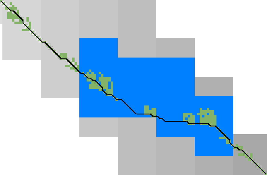
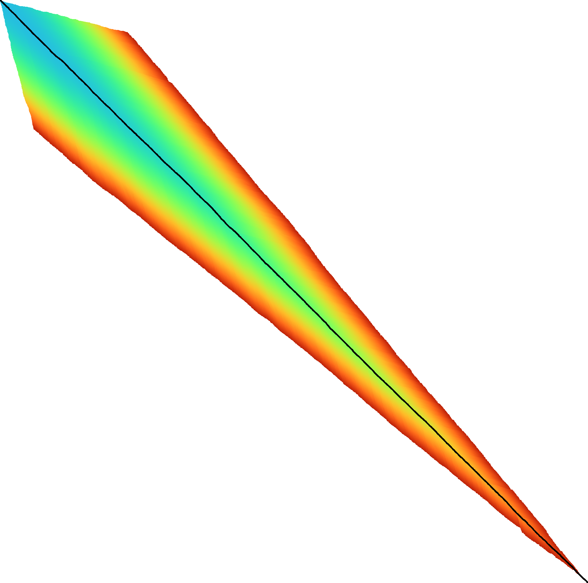
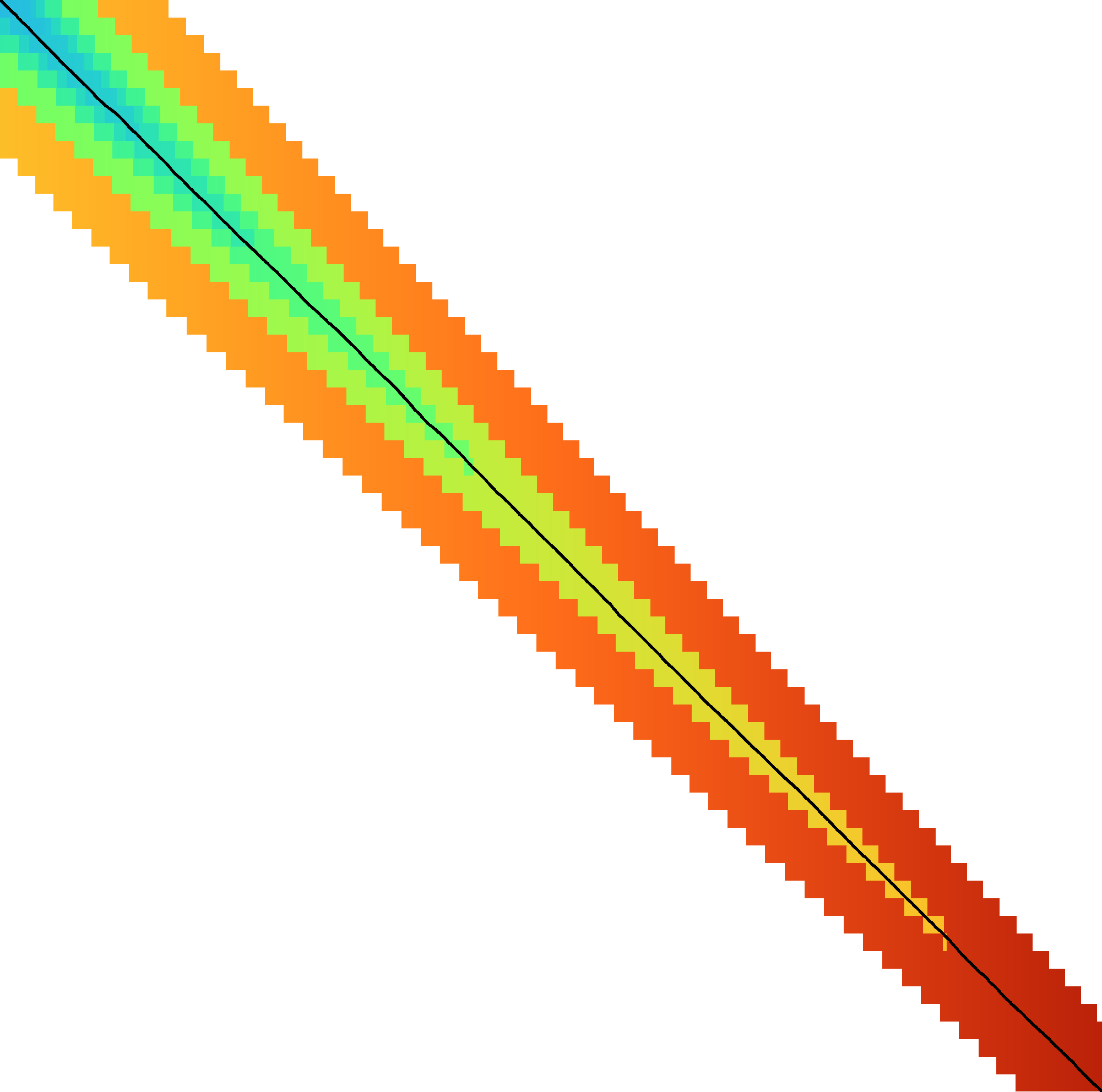
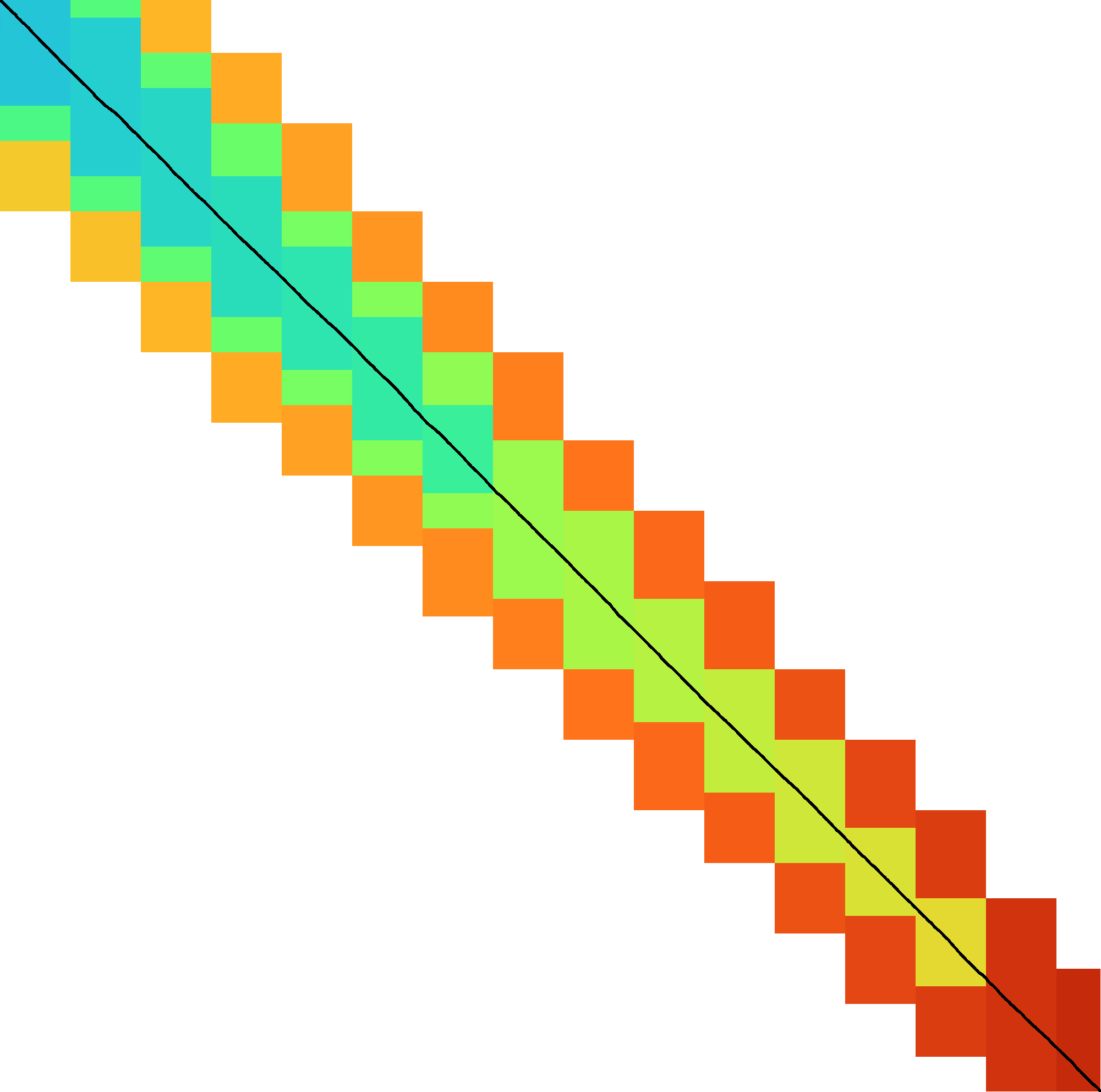
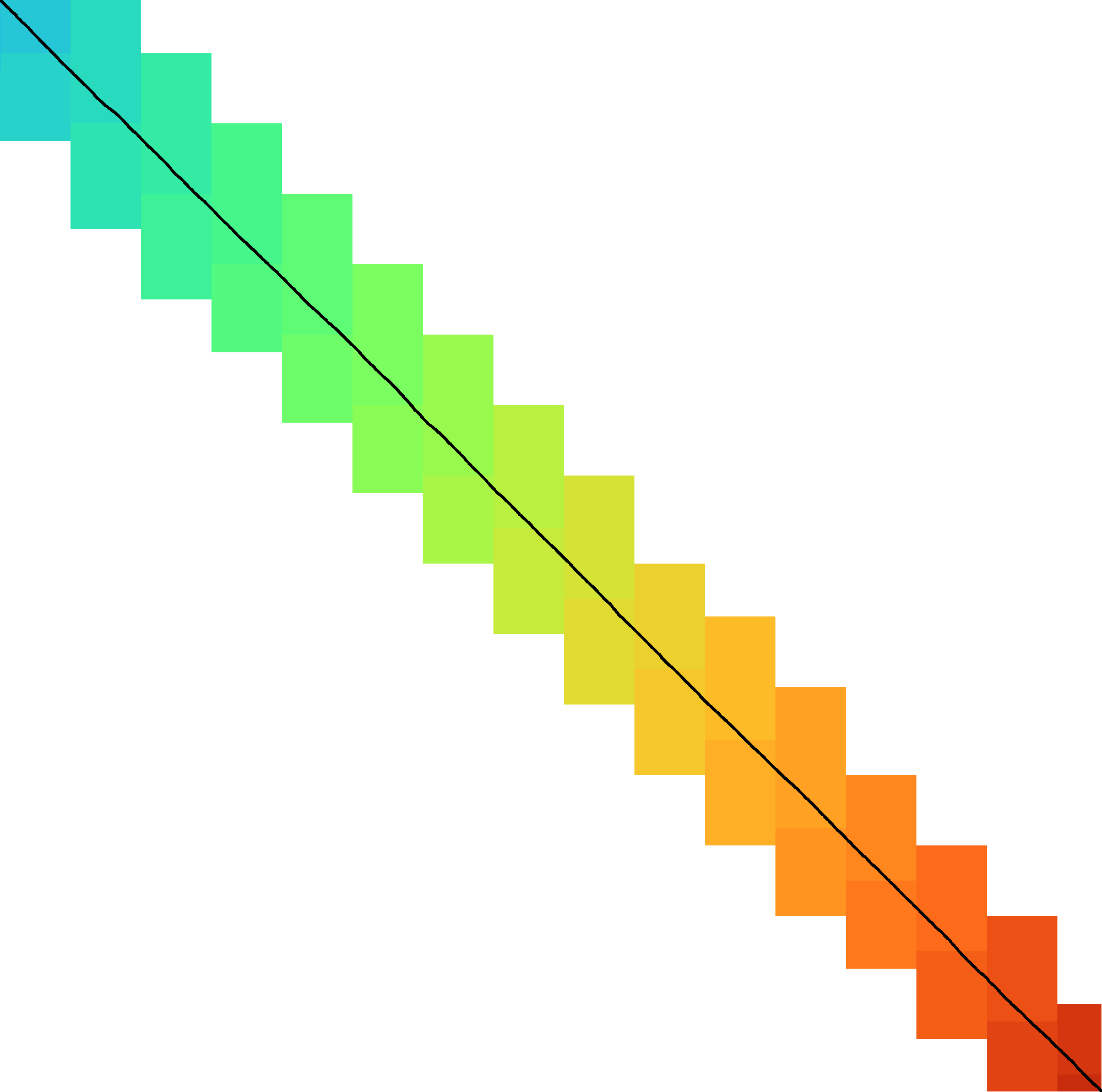
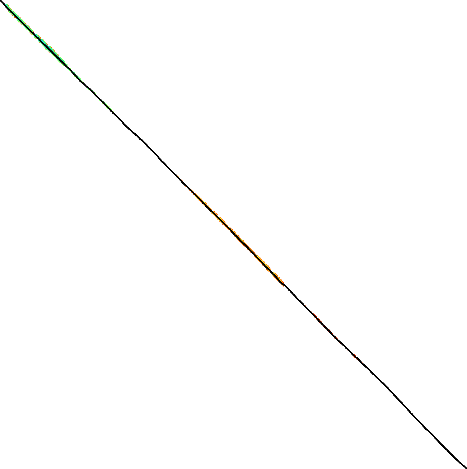
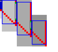
Figure 3: Traceback method. States expanded by the diagonal transition traceback in each block are shown in green. When the distance in a block is too large, a part of the block is fully recomputed as fallback, as shown in blue.
The traceback stage takes as input the computed vertical differences at the end of each block of columns. We iteratively work backwards through the blocks. In each step, we know the distances \(g(\st ij)\) to the states in column \(i\) and the state \(u=\st{i+B}j\) in column \(i+B\) that is on the optimal path and has distance \(\g(u)\). The goal is to find an optimal path from column \(i\) to \(u\).
A naive approach is to simply recompute the entire block of columns while storing distances to all states. Here we consider two more efficient methods.
Optimistic block computation. Instead of computing the full range for this column, a first insight is that only rows up to \(j\) are needed, since the optimal path to \(u=\st{i+B}j\) can never go below row \(j\).
Secondly, the path crosses \(B=256\) columns, and so we optimistically assume that it will be contained in rows \(j-256-64=j-320\) to \(j\). Thus, we first compute the distance to all states in this range of rows (rounded out to multiples of \(w=64\)). If the distance to \(u\) computed this way agrees with the known distance, there is a shortest path contained within the computed rows and we trace it one state at a time. Otherwise, we repeatedly try again with double the number of lanes, until success. The exponential search ensures low overhead and good average case performance.
Optimistic diagonal transition traceback (DTT). A second improvement uses the diagonal transition algorithm backwards from \(u\). We simply run the unmodified algorithm on the reverse graph covering columns \(i\) to \(i+B\) and rows \(0\) to \(j\). Whenever a state \(v\) in column \(i\) is reached, with distance \(d\) from \(u\), we check whether \(g(v) + d=\g(u)\), and continue until a \(v\) is found for which this holds. We then know that \(v\) lies on a shortest path and can find the path from \(v\) to \(u\) by a usual traceback on the diagonal transition algorithm.
As an optimization, when no suitable \(v\) is found after trying all states at distance \(\leq 40\), we abort the DTT and fall back to the block doubling described above. Another optimization is the WF-adaptive heuristic introduced by WFA: all states that lag more than \(10\) behind the furthest reaching diagonal are dropped. Lastly, we abort early when after reaching distance \(20=40/2\), less than half the columns were reached.
Figure 3 shows that in regions with low divergence, the DTT is sufficient to trace the path, and only in noisy regions the algorithm falls back to recomputing full blocks.
3.7 A* Link to heading
Edlib already uses a simple gap-cost heuristic that gives a lower bound on the number of insertions and deletions on a path from each state to the end. We replace this by the much stronger gap-chaining seed heuristic (GCSH) introduced in A*PA.
Compared to A*PA, we make two modifications.
3.7.1 Bulk-contours update Link to heading
In A*PA, matches are pruned as soon as a shortest path to their start has been found. This helps to penalize states before (left of) the match. Each iteration of our new algorithm works left-to-right only, and thus pruning of matches does not affect the current iteration. Instead of pruning on the fly, we collect all matches to be pruned at the end of each iteration, and update the contours in one right-to-left sweep.
To ensure the band doubling approach remains valid after pruning, we ensure that the range of computed rows never shrinks after an increase of \(t\) and subsequent pruning.
3.7.2 Pre-pruning Link to heading
 |  |
Here we introduce an independent optimization that also applies to the original A*PA method.
Each of the heuristics \(h\) introduced in A*PA depends on the set of matches \(\matches\). Given that \(\matches\) contains all matches, \(h\) is an admissible heuristic that never overestimates the true distance. Even after pruning some matches, \(h\) is still a lower bound on the length of a path not going through already visited states.
Now consider an exact match \(m\) from \(u\) to \(v\) for seed \(s_i\). The existence of the match is a ‘promise’ that seed \(s_i\) can be crossed for free. When \(m\) is a match outside the optimal alignment, it is likely that \(m\) can not be extended into a longer alignment. When indeed \(m\) can not be extended into an alignment of \(s_i\) and \(s_{i+1}\) of cost less than \(2\), the existence of \(m\) was a ‘false promise’, since crossing the two seeds takes cost at least \(2\). Thus, we can ignore \(m\) and remove \(m\) from the heuristic, making the heuristic more accurate.
More generally, we try to extend each match \(m\) into an alignment covering seeds \(s_i\) up to (but excluding) \(s_{i+q}\) for all \(q\leq p=14\). If any of these extensions has cost at least \(q\), i.e. \(m\) falsely promised that \(s_i\) to \(s_{i+q}\) can be crossed for cost \(<q\), we pre-prune (remove) \(m\).
We try to extend each match by running the diagonal transition algorithm from the end of each match, and dropping any furthest reaching points that are at distance \(\geq q\) while at most \(q\) seeds have been covered.
As shown in Table 2b, the effect is that the number of off-path matches is significantly reduced. This makes contours faster to initialize, update, and query, and increases the value of the heuristic
3.8 Determining the rows to compute Link to heading
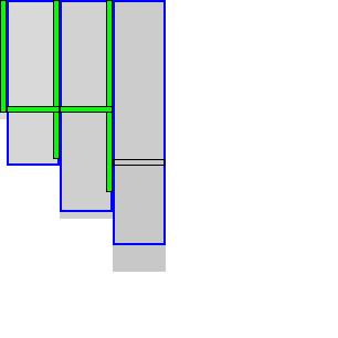
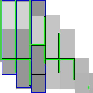
For each block spanning columns \(i\) to \(i+B\), only a subset of rows is computed in each iteration. Namely, we only compute those rows that can possibly contain states on a path/alignment of cost at most \(t\). Intuitively, we try to ’trap’ the alignment inside a wall of states that can not lie on a path of length at most \(t\) (i.e. have \(\f(u) \geq t\)), as can be seen in Table 3a. We determine this range of rows in two steps:
- First, we determine the fixed range at the end of the preceding block. I.e., we find the topmost and bottom-most states \(\st i{j_{start}}\) and \(\st i{j_{end}}\) with \(f(u) = g(u) + h(u) \leq t\). All in-between states \(u=\st ij\) with \(j_{start}\leq j\leq j_{end}\) are then fixed, meaning that the correct distance has been found and \(g(u) = \g(u)\).
- Then, we use the heuristic to find the bottom-most state \(v=\st{i+B}{j_{end}’}\) at the end of the to-be-computed block that can possibly lie on a path of length \(\leq t\). We then compute rows \(j_{start}\) to \(j_{end}’\) in columns \(i\) to \(i+B\), rounding \([j_{start}, j_{end}’]\) out to the previous/next multiple of the word size \(w=64\).
Step 1: Fixed range. Suppose that states in rows \([r_{start}, r_{end}]\) were computed. One way to find \(j_{start}\) and \(j_{end}\) is by simply iterating inward from the start/end of the range and dropping all states with \(f(u)=g(u)+h(u)>t\), as indicated by the red columns in Table 3a.
Step 2: End of computed range. We will now determine the bottom-most row \(j\) that can contain a state at distance \(\leq t\) at the end of the block. Let \(u=\st{i}{j_{end}}\) be the bottom-most fixed state in column \(i\) with distance \(\leq t\). Let \(v = \st{i’}{j’}\) be a state in the current block (\(i\leq i’\leq i+B\)) that is below the diagonal of \(u\). Suppose \(v\) lies on a path of length \(\leq t\). This path most cross column \(i\) in or above \(u\), since states \(u’\) below \(u\) have \(\f(u’)>t\). The distance to \(v\) is now at least \(\min_{j\leq j_{end}} \g(\st ij) + \cgap(\st ij, v) \geq \g(u) + \cgap(u, v)\), and thus we define \[ f_l(v) := \g(u) + \cgap(u,v) + h(v) \] as a lower bound on the length of the shortest path through \(v\), assuming \(v\) is below the diagonal of \(u\) and \(\f(v) \leq t\). When \(f_l(v)>t\), this implies \(\f(v)>t\) and also \(\f(v’) > t\) for all \(v’\) below \(v\).
The end of the range is now computed by finding the bottom-most state \(v\) in each column for which \(f_l\) is at most \(t\), using the following algorithm (omitting boundary checks).
- Start with \(v = \st{i’}{j’} = u = \st{i}{j_{end}}\).
- While the below-neighbour \(v’ = \st{i’}{j’+1}\) of \(v\) has \(f_l(v)\leq t\), increment \(j’\).
- Go to the next column by incrementing \(i’\) and \(j’\) by \(1\) and repeat step 2, until \(i’=i+B\).
The row \(j’_{end}\) of the last \(v\) we find in this way is the bottom-most state in column \(i+B\) that can possibly have \(f(v)\leq t\), and hence this is end of the range we compute.
In Table 3a, we see that \(f(v)\) is evaluated at a diagonal of states just below the bottommost green (fixed) state \(u\) at the end of the preceding black, and that the to-be-computed range (indicated in blue) includes exactly all states above the diagonal.
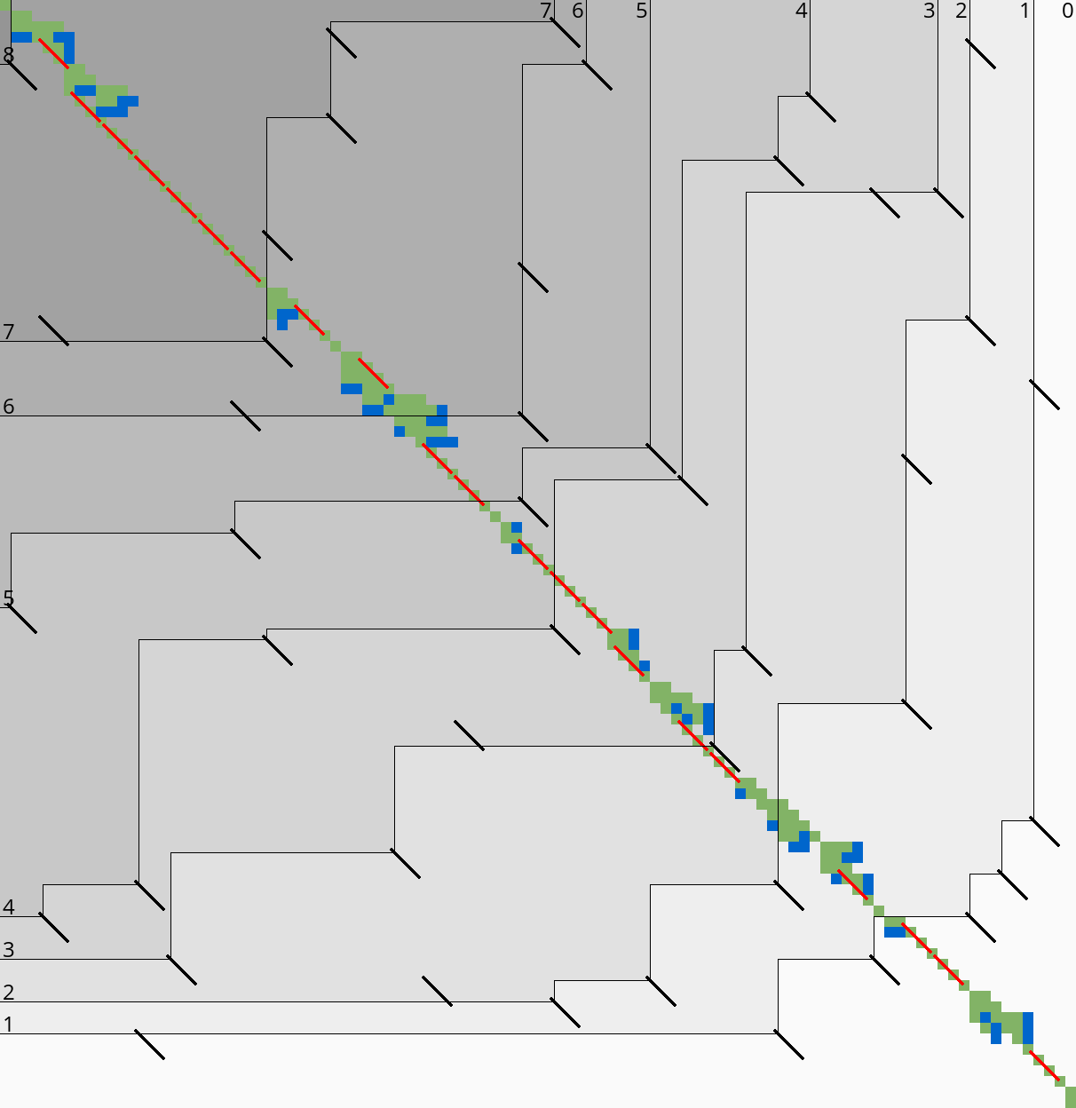
 Simple Simple | 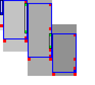 Sparse Sparse |
3.8.1 Sparse heuristic invocation Link to heading
A drawback of the previous method is that it requires a large number of calls to \(f\) and hence the heuristic \(h\): roughly one per column and one per row. Here we present a sparse version that uses fewer calls to \(f\), based on two similar lemmas.
Lemma 1. When \(h\) is admissible and \(f(u) > t + 2D\), then \(\f(u’) > t\) when \(d(u, u’) \leq D\).
Proof. Since adjacent states differ in distance by \(\{-1,0,+1\}\), we have \(g(u’) \geq g(u) - d(u,u’) \geq g(u)-D\) and \(\h(u’) \geq \h(u’) - d(u,u’) \geq \h(u)-D\). Now suppose that \(\f(u’) \leq t\). Then \(u’\) is fixed and we have \(g(u’) = \g(u’)\), and since \(h\) is admissible \(h(u’) \leq \h(u’)\). Thus:
\begin{align*} f(u) &= g(u ) + h(u)\\ &\leq g(u ) + \h(u) \leq g(u’) + \h(u’) + 2D\\ &= \g(u’) + \h(u’) + 2D = \f(u’) + 2D \leq t + 2D. \end{align*}
This is in contradiction with \(f(u) > t+2D\), so we must have \(\f(u’) > t\), as required.
Lemma 2. When \(h\) is admissible, \(v\) is below the diagonal of a computed state \(u\), and \(f_l(v) = \g(u) + \cgap(u,v)+h(v) > t + 2D\), then \(\f(v’) > t\) when \(d(v,v’) \leq D\).
Proof. We have \(\cgap(u, v’) \geq \cgap(u,v) - d(v,v’) \geq \cgap(u,v)-D\), and \(\h(v’) \geq \h(v)-D\). From before we already know that \(\g(u) + \cgap(u,v) \leq \g(v)\), and we still have \(h(v) \leq \h(v)\) and \(\g(v’) \geq \g(v) - D\) and \(\h(v’) \geq \h(v) -D\). The result follows directly:
\begin{align*} t < f_l(v) - 2D &=\g(u ) + \cgap(u,v) + h(v) -2D\\ &\leq \g(v) + \h(v)-2D \leq \g(v’) + \h(v’) = \f(v’). \end{align*}
Sparse fixed range. To find the first row \(j_{start}\) with \(f(\st i{j_{start}})\leq t\), start with \(j=r_{start}\), and increment \(j\) by \(\lceil(f(v)-t)/2\rceil\) as long as \(f(v)>t\), since none of the intermediate states can lie on a path of length \(\leq t\) by Lemma 1. The last row is found in the same way. As seen in Table 3b, this sparse variant significantly reduces the number of evaluations of the heuristic in the right-most columns of each block.
Sparse end of computed range. Lemma 2 inspires the following algorithm (Table 3b). Instead of considering one column at a time, we now first make a big just down and then jump to the right.
- Start with \(v = \st{i’}{j’} = u+\st{1}{B+1} = \st{i+1}{j_{end} + B+1}\).
- If \(f_l(v) \leq t\), increase \(j’\) (go down) by \(8\).
- If \(f_l(v) > t\), increase \(i’\) (go right) by \(\lceil(f_l(v)-t)/2\rceil\), but do not exceed column \(i+B\).
- Repeat from step 2, until \(i’ = i+B\).
- While \(f_l(v) > t\), decrease \(j’\) (go up) by \(\lceil(f_l(v)-t)/2\rceil\), but do not go above the diagonal of \(u\).
The resulting \(v\) is again the bottom-most state in column \(i+B\) that can potentially have \(f(t)\leq t\), and its row is the last row that will be computed.
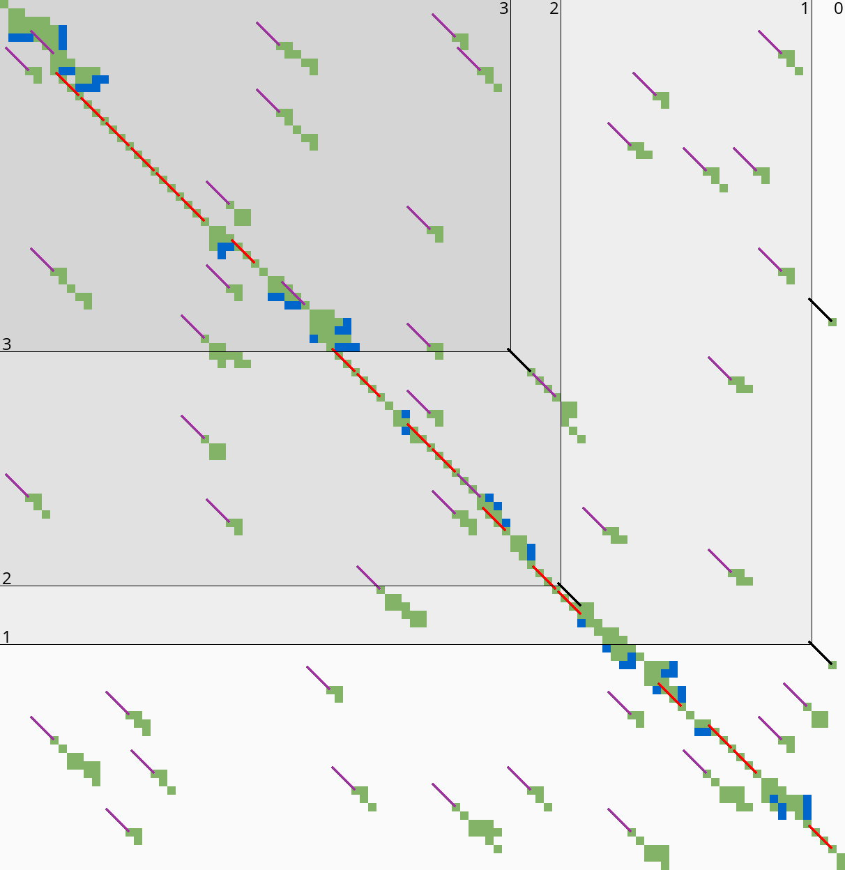
3.9 Incremental doubling Link to heading
 |  |
When the original band doubling algorithm doubles the threshold from \(t\) to \(2t\), it simply recomputes the distance to all states. On the other hand, BFS, Dijkstra, and A* with a consistent heuristic visit states in increasing order of distance (\(g(u)\) for BFS and Dijkstra, \(f(u) = g(u) + h(u)\) for A*), and the distance to a state is known to be correct (fixed) as soon as it is expanded. This way a state is never expanded twice.
Indeed, our band-doubling algorithm can also avoid recomputations. After completing the iteration for \(t\), it is guaranteed that the distance is fixed to all states that indeed satisfy \(f(u)\leq t\). In fact a stronger result holds: in any column the distance is fixed for all states between the topmost and bottom-most state in that column with \(f(u)\leq t\).
To be able to skip rows, we must store horizontal differences along a row so we can continue from there. We choose this row \(j_f\) (for fixed) as the last row at a lane boundary before the end of the fixed states in the last column of the preceding block, as indicated in Table 4 by a horizontal black rectangle. In the first iteration, reusing values is not possible, so we split the computation of the block into two parts (Table 4a): one above \(j_h\), to extract and store the horizontal differences at \(j_h\), and the remainder below \(j_h\).
In the second and further iterations, the values at \(j_h\) may be reused and the block is split into three parts. The first part computes all lanes covering states before the start of the already-fixed range at the end of the block (the green column at the end of the third column in Table 4b). Then we skip the lanes up to the previous \(j_h\), since the values at both the bottom and right of this region are already fixed. Then, we compute the lanes between the old \(j_h\) and its new value \(j’_h\). Lastly we compute the lanes from \(j’_h\) to the end.
4 Results Link to heading
Our implementation A*PA is written in Rust and available at github.com/RagnarGrootKoerkamp/astar-pairwise-aligner. We compare it against other aligners on real datasets, report the impact of the individual techniques we introduced, and measure time and memory usage.
4.1 Setup Link to heading
Datasets. We benchmark on six datasets containing real sequences of varying length and divergence, as listed in detail in 6.2. They can be downloaded from github.com/pairwise-alignment/pa-bench/releases/tag/datasets.
Four datasets containing Oxford Nanopore Technologies (ONT) reads are reused from the WFA, BiWFA, and A*PA evaluations (Marco-Sola et al. 2021, 2023; Groot Koerkamp and Ivanov 2024). Of these, the ‘>500kbp’ and ‘>500kbp with genetic variation’ datasets have divergence \(6-7\%\), while two ‘1kbp’ and ‘10kbp’ datasets are filtered for sequences of length <1kbp and <50kbp have average divergence \(11\%\) and average sequence length $800$bp and $11$kbp.
A SARS-CoV-2 dataset was newly generated by downloading 500MB of viral sequences from the COVID-19 Data Portal, covid19dataportal.org (Harrison et al. 2021), filtering out non-ACTG characters, and selecting \(10000\) random pairs. This dataset has average divergence \(1.5\%\) and length $30$kbp.
For each set, we sorted all sequence pairs by edit distance and split them into \(50\) files each containing multiple pairs, with the first file containing the \(2\%\) of pairs with the lowest divergence. Reported results are averaged over the sequences in each file.
Algorithms and aligners. We benchmark A*PA2 against state-of-the-art exact aligners Edlib, BiWFA, and A*PA. We further compare against the approximate aligners WFA-Adaptive (Marco-Sola et al. 2021) and Block Aligner. For WFA-Adaptive we use default parameters \((10, 50, 10)\), dropping states that lag behind by more than \(50\). For Block Aligner we use block sizes from \(0.1\%\) to \(1\%\) of the input size. Block Aligner only supports affine costs so we use gap-open cost \(1\) instead of \(0\).
We compare two versions of A*PA2. A*PA2-simple uses all engineering optimizations (bitpacking, SIMD, blocks, new traceback) and uses the simple gap-heuristic. A*PA2-full additionally uses more complicated techniques: incremental-doubling, and the gap-chaining seed heuristic introduced by A*PA with pre-pruning.
Parameters. For A*PA2, we fix block size \(B=256\). For A*PA2-full, we use the gap-chaining seed heuristic (GCSH) of A*PA with exact matches (\(r=1\)) and seed length \(k=12\). We pre-prune matches by looking ahead up to \(p=14\) seeds. A detailed parameter comparison can be found in 6.2. For A*PA, we use inexact matches (\(r=2\)) with seed length \(k=15\) by default, and only change this for the low-divergence SARS-CoV-2 dataset and \(4\%\) divergence synthetic data, where we use exact matches (\(r=1\)) instead.
Execution.
We ran all benchmarks using PaBench (github.com/pairwise-alignment/pa-bench) on
Arch Linux on an Intel Core i7-10750H with $64$GB of memory and \(6\) cores,
with hyper-threading disabled, frequency boost disabled, and CPU power saving
features disabled. The CPU frequency is fixed to $3.3$GHz and we run \(1\)
single-threaded job at a time with niceness \(-20\). Reported running times are
the average wall-clock time per alignment and do not include the time to read
data from disk. For A*PA2-full, reported times do include the time to find matches and
initialize the heuristic.
4.2 Comparison with other aligners Link to heading
Speedup on real data. Figure 4 compares the running time of aligners on real datasets. 6.2 contains a corresponding table of average runtimes. For long ONT reads, with \(6\%-7\%\) divergence, A*PA2-full is \(19\times\) faster than Edlib, BiWFA, and A*PA in average running time, and using the gap-chaining seed heuristic in A*PA2-full provides speedup over A*PA2-simple.
On shorter sequences, the overhead of initializing the heuristic in A*PA2-full is large, and A*PA2-simple is faster. For the 10kbp dataset, A*PA2-simple is \(5.6\times\) faster than other exat methods. For the shortest (<1kbp ONT reads) and most similar sequences (SARS-CoV-2 with \(1\%\) divergence), BiWFA is usually faster than Edlib and A*PA2-simple. In these cases, the overhead of using \(256\) wide blocks is relatively large compared to the edit distance \(s\leq 500\) in combination with BiWFAs \(O(s^2+n)\) expected running time.

Figure 4: Runtime comparison (log). Each dot shows the running time of a single alignment (right two plots) or the average runtime over (2%) of the input pairs (left four plots). Box plots show the three quartiles, and the red circled dot shows the average running time over all alignments. For APA, exact matches ((r=1)) are used for the SARS-CoV-2 dataset, some alignments $≥10$kbp time out, and the shown average is a lower bound on the true average. Approximate aligners WFA Adaptive and Block Aligner are indicated with a triangle. On the >500kbp reads, APA2-full is (20times) faster than other methods.
Comparison with approximate aligners. For the smallest datasets, BiWFA is about as fast as the approximate methods WFA Adaptive and Block Aligner, while for the largest datasets A*PA2-full is significantly faster. Only for the set of $10$kbp ONT reads is Block Aligner significantly (\(\approx 2\times\)) faster than the fastest exact method. For the two smallest datasets, approximate aligners do not significantly improve on BiWFA. Only on the $10$kbp ONT reads dataset is Block Aligner \(1.6\times\) faster than A*PA2, but it only reports \(53\%\) of the alignments correctly. All accuracy numbers can be found in 6.2.
Scaling with divergence. Table 5 compares the runtime of aligners on synthetic sequences of increasing divergence. BiWFA’s runtime grows quadratically, while Edlib grows linearly and jumps up each time another doubling of the threshold is required. A*PA is fast until the maximum potential is reached at \(6\%\) resp. \(12\%\) and then becomes very slow. A*PA2 behaves similar to Edlib and jumps up each time another doubling of the threshold is needed, but is much faster. It outperforms BiWFA for divergence \(\geq 2\%\) and A*PA for divergence \(\geq 4\%\). The runtime of A*PA2-full is near-constant up to divergence \(7\%\) due to the gap-chaining seed heuristic which can correct for up to \(1/k=1/12=8.3\%\) of divergence, while A*PA2-simple starts to slow down because of doubling at lower divergence. For a fixed number of doublings of the threshold, A*PA2 is faster for higher divergence because too low thresholds are rejected more quickly.
 |  |
Scaling with length. Table 6 compares the runtime of aligners on synthetic random sequences of increasing length and constant uniform divergence. BiWFA’s runtime is quadratic and is fast for sequences up to $3000$bp. As expected, A*PA2-simple has very similar scaling to Edlib but is faster by a constant factor. A*PA2-full includes the gap-chaining seed heuristic used by A*PA, resulting in comparable speed and near-linear scaling for both of them when \(d=4\%\). For more divergent sequences, A*PA2-full is faster than A*PA since initializing the A*PA heuristic with inexact matches is relatively slow. The reason A*PA2-full is slower than A*PA for sequences of length $10$Mbp is that A*PA2-full uses seed length \(k=12\) instead of \(k=15\), causing the number of matches to explode when \(n\) approaches \(4^{12}\approx 16 \cdot 10^6\).
 |  |
Memory usage of A*PA2 on >500kbp sequences is at most $200$MB and $30$MB in median. For shorter sequences, memory usage is always less than $10$MB (6.2).
4.3 Effects of methods Link to heading
Incremental improvements. Figure 5 shows the effect of one-by-one adding improvements to A*PA2 on >500kbp long sequences, starting with Ukkonen’s band-doubling method using Myers’ bitpacking. We first change to the \(\g(u) + \cgap(u, v_t)\) domain, making it comparable to Edlib. Then we process blocks of \(256\) columns at a time and only store differences at block boundaries giving \(\approx 2\times\) speedup. Adding SIMD gives another \(\approx 3\times\) speedup, and instruction level parallelism (ILP) provides a further small improvement. The diagonal transition traceback (DTT) and sparse heuristic computation do not improve performance of A*PA2-simple much on long sequences, but their removal can be seen to slow it down for shorter sequences in Figure 7.
Incremental doubling (ID), the gap-chaining seed heuristic (GCSH), pre-pruning (PP), and the pruning of A*PA give another \(2\times\) speedup on average and \(3\times\) speedup in the first quantile.

Figure 5: Effect of adding features. Box plots showing the performance improvements of APA2 when incrementally adding new methods one-by-one. APA2-simple corresponds to the rightmost red columns, and A*PA2-full corresponds to the rightmost blue column.
Runtime profile. In Figure 6 we see that for >500kbp long sequences, A*PA2-full spends most of its time computing blocks, followed by the initialization of the heuristic. For shorter sequences the heuristic is not used, and for very short sequences <10kbp, up to half the time is spent on tracing the optimal alignment.

Figure 6: Runtime distribution per stage of A*PA2, using APA2-simple for short sequences and APA2-full for the two rightmost >500kbp datasets. Each column corresponds to a (set of) alignment(s), which are sorted by total runtime. Overhead is the part of the runtime not measured in one of the other parts and includes the time to build the profile.
5 Discussion Link to heading
We have shown that by incorporating many existing techniques and by writing highly performant code, A*PA2 achieves \(19\times\) speedup over other methods when aligning $>500$kbp ONT reads with \(6\%\) divergence, \(5.6\times\) speedup for sequences of average length \(11\) kbp, and only a slight slowdown over BiWFA for very short (\(<1000\) bp) and very similar (\(<2\%\) divergence) sequences. A*PA2’s speed is also comparable to approximate aligners, and is faster for long sequences, thereby nearly closing the gap between approximate and exact methods. A*PA2 achieves this by building on Edlib, using band doubling, bitpacking, blocks, SIMD, the gap-chaining seed heuristic, and pre-pruning. The effect of this is that A*PA2-simple has similar scaling behaviour as Edlib in both length and divergence, but with a significantly better constant. A*PA2-full additionally includes the A*PA heuristics and achieves the best of both worlds: the near-linear scaling with length of A*PA when divergence is small, and the efficiency of Edlib.
Limitations.
- The main limitation of A*PA2-full is that the heuristic requires finding all matches between the two input sequences, which can take long compared to the alignment itself.
- For sequences with divergence \(<2\%\), BiWFA exploits the sparse structure of the diagonal transition algorithm. In comparison, computing full blocks of size around \(256\times 256\) in A*PA2 has considerable overhead.
- Only sequences over alphabet size \(4\) are currently supported, so DNA
sequences containing e.g.
Ncharacters must be cleaned first.
Future work.
- When divergence is low, performance could be improved by applying A* to the diagonal transition algorithm directly, instead of using DP. As a middle ground, it may be possible to compute individual blocks using DT when the divergence is low.
- Currently A*PA2 is completely unaware of the type of sequences it aligns. Using an upper bound on the edit distance, either known or found using a non-exact method, could avoid trying overly large thresholds and smoothen the curve in Table 5.
- It should be possible to extend A*PA2 to open-ended and semi-global alignment, just like Edlib and WFA support these modes.
- Extending A*PA2 to affine cost models should also be possible. This will require adjusting the gap-chaining seed heuristic, and changing the computation of the blocks from a bitpacking approach to one of the SIMD-based methods for affine costs.
- Lastly, TALCO (Tiling ALignment using COnvergence of traceback pointers, https://turakhia.ucsd.edu/research/) provides an interesting idea: it may be possible start traceback while still computing blocks, thereby saving memory.
Acknowledgements Link to heading
I am grateful to Daniel Liu for discussions, feedback, and suggesting additional related papers, to André Kahles, Harun Mustafa, and Gunnar Rätsch for feedback on the manuscript, to Andrea Guarracino and Santiago Marco-Sola for sharing the WFA and BiWFA benchmark datasets, and to Gary Benson for help with debugging the BitPAl bitpacking code. RGK is financed by ETH Research Grant ETH-1721-1 to Gunnar Rätsch.
Conflict of interest Link to heading
None declared.
6 Appendix Link to heading
6.1 Bitpacking Link to heading
Code Snippet 1 shows a SIMD version of Myers’ bitpacking algorithm, and Code Snippet 2 shows a SIMD version of the edit distance bitpacking scheme explained in the supplement of Loving, Hernandez, and Benson (2014). Both methods require \(20\) instructions.
Both methods are usually reported to use fewer than \(20\) instructions, but exclude the shifting out of the bottom horizontal difference (four instructions) and the initialization of the carry for BitPAl (one operation). We require these additional outputs/inputs since we want to align multiple $64$bit lanes below each other, and the horizontal difference in between must be carried through.
| |
| |
6.2 Comparison with other aligners Link to heading
Here we provide further results on the comparison of aligners.
Dataset statistics. Detailed statistics on the datasets are provided in Table 7. The ONT (Oxford Nanopore Technologies) read sets all have high \(6\%-12\%\) divergence, and the set with genetic variation (gen.var.) contains long gaps. The SARS-CoV-2 dataset stands out for having only \(1.5\%\) divergence.
| Dataset | Source | #Pairs | len min | len mean | len max | div min | div mean | div max | max gap mean | max gap max |
|---|---|---|---|---|---|---|---|---|---|---|
| SARS-CoV-2 | A*PA2 | 10000 | 27 | 30 | 30 | 0.0 | 1.5 | 12.8 | 0.1 | 1.0 |
| ONT <1k | WFA | 12477 | 0.04 | 0.8 | 1.1 | 0.0 | 10.4 | 22.5 | 0.01 | 0.1 |
| ONT <10k | BiWFA | 5000 | 0.2 | 3.6 | 10 | 3.0 | 12.1 | 20.1 | 0.04 | 0.5 |
| ONT <50k | BiWFA | 10000 | 0.2 | 11 | 50 | 3.0 | 11.6 | 19.2 | 0.07 | 3.4 |
| ONT >500k | A*PA | 50 | 500 | 594 | 849 | 2.7 | 6.1 | 16.7 | 0.1 | 1.3 |
| ONT >500k + gen.var. | BiWFA | 48 | 502 | 632 | 1053 | 4.3 | 7.2 | 18.2 | 1.9 | 42 |
Runtime comparison on real data. Table 8 shows the numeric value of the average runtime of each aligner in Figure 4.
| SARS-CoV-2 pairs (ms) | 1kbp ONT reads (ms) | 10kbp ONT reads (ms) | >500kbp ONT reads (s) | >500kbp ONT reads + gen.var. (s) | |
|---|---|---|---|---|---|
| Edlib | 11.14 | 0.110 | 8.0 | 3.74 | 5.20 |
| BiWFA | 1.13 | 0.042 | 9.3 | 4.47 | 6.96 |
| A*PA | 6.25 | 0.514 | >190.1 | >14.01 | >12.92 |
| WFA Adaptive | 0.85 | 0.038 | 3.0 | 1.04 | 0.81 |
| Block Aligner | 2.35 | 0.038 | 0.9 | 0.63 | 0.68 |
| A*PA2 simple | 0.89 | 0.052 | 1.4 | 0.58 | 0.78 |
| A*PA2 full | 2.00 | 0.083 | 1.7 | 0.20 | 0.27 |
| Speedup | 1.3× | 0.81× | 5.6× | 18.8× | 19.0× |
Approximate aligner accuracy. Table 9 shows the percentage of alignments in each dataset for which approximate methods report the correct distance. The accuracy of WFA Adaptive drops a lot for the >500kbp dataset with genetic variation, since these alignments contain gaps of thousands of basepairs, much larger than the $50$bp cutoff after which trailing diagonals are dropped.
| SARS-CoV-2 pairs | 1kbp ONT reads | 10kbp ONT reads | >500kbp ONT reads | >500kbp ONT reads + gen.var. | |
|---|---|---|---|---|---|
| WFA Adaptive | 92 | 93 | 49 | 60 | 4 |
| Block Aligner | 34 | 85 | 53 | 96 | 50 |
Memory usage. Table 10 shows the memory usage of all compared aligners.
max_rss before and after aligning a pair of sequences.| Memory [MB] | SARS-CoV-2 pairs Median | SARS-CoV-2 pairs Max | 1kbp ONT reads Median | 1kbp ONT reads Max | 10kbp ONT reads Median | 10kbp ONT reads Max | >500kbp ONT reads Median | >500kbp ONT reads Max | >500kbp ONT reads + gen.var. Median | >500kbp ONT reads + gen.var. Max |
|---|---|---|---|---|---|---|---|---|---|---|
| Edlib | 0 | 0 | 0 | 0 | 0 | 0 | 0 | 0 | 0 | 0 |
| BiWFA | 0 | 0 | 0 | 0 | 0 | 0 | 4 | 11 | 0 | 2 |
| A*PA | 0 | 236 | 0 | 0 | 228 | 873 | 84 | 3453 | 158 | 6868 |
| WFA Adaptive | 0 | 11 | 0 | 0 | 0 | 0 | 0 | 0 | 0 | 0 |
| Block Aligner | 0 | 16 | 0 | 0 | 0 | 3 | 583 | 1189 | 610 | 2171 |
| A*PA2 simple | 2 | 5 | 0 | 0 | 4 | 6 | 0 | 55 | 2 | 164 |
| A*PA2 full | 0 | 0 | 0 | 0 | 0 | 0 | 30 | 82 | 6 | 141 |
6.3 Effects of methods Link to heading
Ablation. Figure 7 shows how the performance of A*PA2 changes as individual features are removed.

Figure 7: Ablation. Box plots showing how the performance of APA2-simple and APA2-full changes when removing features.
Parameters. Figure 8 compares A*PA2 with default parameters against versions where one of the parameters is modified. As can be seen, running time is not very sensitive with regards to most parameters. Of note are using inexact matches (\(r=2\)) for the heuristic, which take significantly longer to find, larger seed length \(k\), which decreases the strength of the heuristic, and smaller block sizes (\(B=128\) and \(B=64\)), which induce more overhead.

Figure 8: Changing parameters. Running time of APA2-simple (left, middle) and APA2-full (right) with one parameter modified. Default parameters are seed length (k=12), pre-pruning look-ahead (p=14), growth factor (f=2), block size (b=256), max traceback cost (g=40), and dropping diagonals that lag (fd=10) behind during traceback.