- 1 Optimizing Binary Search And Interpolation Search
- 2 Binary search
- 3 Eytzinger
- 3.1 Naive implementation
- 3.2 Prefetching
- 3.3 Branchless Eytzinger
- 3.4 Batched Eytzinger
- 3.4.1 Non-prefetched
- 3.4.2 Prefetched
- 4 Eytzinger or BinSearch?
- 5 Memory efficiency – parallel search and comparison to S-trees
- 6 Interpolation search
- 7 Conclusion and takeaways
1 Optimizing Binary Search And Interpolation Search Link to heading
This blogpost is a preliminary of the post on static search trees. We will be looking into binary search and how it can be optimized using different memory layouts (Eytzinger), branchless techniques and careful use of prefetching. In addition, we will explore batching. Our language of choice will be Rust.
The goal of this text is mainly educational, as we’ll mostly be replicating research that has already been done. Looking at performance plots is fun!
The source code can be found at https://github.com/RagnarGrootKoerkamp/static-search-tree.
1.1 Problem statement Link to heading
Input: we take a sorted array of n unsigned 32-bit integers.
Output: for a query q, find the smallest element >= q or u32::MAX
if no such element exists.
Metric: we optimize throughput. In plots, we always report amortized time per query (lower is better).
Optimizing for throughput is relevant because for many use-cases, e.g. in bioinformatics, the queries are often independent and the latency is not critical. It also allows for the usage of batching, which helps us hide memory latency.
To be able to easily check implementations against each other,
we always have the largest possible value (u32::MAX) in the input array, so that the result always exists.
1.2 Inspiration and background Link to heading
This article is inspired by a post in Algorithmica on binary search. We start by reimplementing its experiments and expand upon it by optimizing for throughput. We also took inspiration from the notable paper Array Layouts For Comparison-Based Searching by Paul-Virak Khuong and Pat Morin, which goes in-depth on more-or-less successful array layouts. The paper is great because it goes step by step and introduces nice models for why different schemes behave like they behave. It is worth a read! It changed my mind on how a good scientific article should look.
1.3 Benchmarking setup Link to heading
The benchmarking was done using rustc 1.85.0-nightly compiled with the -r flag as well as -C target-cpu=native.
This allows the compiler to make use of architectural specifics of the machine.
The CPU is an AMD Ryzen 4750U, and the DRAM is DDR4-2666. For reproducibility, clock speed
was locked at 1.7GHz and turbo boost and hyperthreading were disabled.
This post is built around plenty of performance plots. We will benchmark in arrays up to a size of 1GB, well beyond the size of L3 cache, to see effects of going to main memory.
All measurements are done 5 times. The lines in plots follow the median, and we show the spread of the 2nd to 4th value (i.e., after discarding the minimum and maximum). Note that the results are sometimes very deterministic and the spread is therefore not very visible. The measurements are done at \(1.17^k\) so as to be similar to Algorithmica. This also mitigates some artifacts of limited cache set associativity which we describe in a later section.
We also allocate the datastructures on 2MB hugepages. This is done to reduce pressure on the TLB.
One thing that I am sorry about are the colors in the plots. In some plots, there will be two lines with the same color; usually it is in the noncritical ones. I made it so that algorithms would keep their color across plots, and that means that sometimes, this happened.
2 Binary search Link to heading
We start with a textbook binary search implementation, and we see if we can replicate the results from Algorithmica. Here’s the code:
| |
Here, self is a SortedVec class, which is a wrapper that allocates the sorted vals array
on hugepages.
We note that by default, Rust wraps all accesses to vectors with bounds
checks. Since we are comparing against C++ implementations and there is
no risk of accessing unallocated memory, we implement the get
function, which performs a Rust unsafe get_unchecked to get rid of the
bounds checks. This will also be the case for all the further
experiments.
So, how does it perform? Let’s compare to the Rust standard library
version (denoted here by binary_search_std):

We can see that our naive version is pretty much the same as the library version, only with the exception of some bumps on the graph.
Checking out the standard library source code, we can see that their implementation already
has some optimizations in place. In the binary_search_by function, we
see the following:
| |
So they do a constant number of iterations instead of early stopping
when the value is found and they try to use the cmov instruction if it
is available in the select_unpredictable function. Both these optimizations are done so that the branch
predictor has an easier time (mispredictions are expensive). The cmov
instruction is useful when the result of the comparison can’t be
reliably predicted (which here it really can’t).1 They are also both
recommended by the Algorithmica post, and make the code effectively branchless.
In addition, they do their accesses to the array without bounds checks, in the same way we do.
Looking at the assembly of the naive version, we see that the compiler has already done some optimizations for us. The branch is replaced by a cmov instruction.
It also makes sense that the naive binary search has bumps on the graph. The compiler cannot make the loop take a fixed number of iterations. Whether
to stop on the final iteration becomes difficult to predict when the array does not have a size of a power of two, and therefore
the code takes longer to run, as the CPU sometimes mispredicts this.
It is notable that when you don’t compile with the target-cpu=native flag, the compiler does not replace the branch with a cmov.
We can see the performance in the following plot:

This replicates the result from the first plot in Algorithmica, where the naive code is much slower on small array sizes
but faster on large array sizes. The fact that it contains a branch allows the branch predictor to pick one possibility and
to start prefetching it. This reduces memory latency, because if the branch predictor
is correct, waiting for this prefetched value will not take such a long time.
When we use a cmov, there is no branch, and so the branch predictor can’t do this.
2.1 Branchless search Link to heading
Now let us implement branchless optimizations ourselves as well and see how we do then. Here’s the code:
| |
When first implementing this, me, being a Rust newbie, immediately went
for the cmov crate, as I was unable to make the compiler generate
the cmov on its own just with an if expression. Trying this, I found
out that it is still plenty slower than the select_unpredictable
function that is used in binary_search_by, so I followed the approach
of the standard library.

We can see that we now surpass the performance of both the naive and the standard library version. Since we do a fixed number of iterations, we can also clearly see “stairs” in the graph with every power of two, as the number of instructions is now pretty much a deterministic function of the input size. As caches make the whole process much faster at small sizes, there are also steps, but they are much smaller.
Our branchless code is faster than the naive version; this makes sense, as our naive code does not have a fixed number of iterations, so there is potential for a branch misprediction, which can take a long time. But why is the branchless code faster than the standard library version at large sizes? They should be conceptually the same; both do a fixed number of iterations and both use a conditional move.
Looking at the graph, it seems like the difference is one extra memory request
or one misprediction. Consulting perf and the standard library source code, we see that their code has an extra difficult-to-predict
condition, e.g. whether the input array actually contains the resulting value or not. Based on that, the return value is either
an Err or an Ok value, and the index packed inside is either the index of the value or the index where the search value could be inserted.
Since our branchless version assumes that the result always exists, we do not have to worry about the equality and therefore do not suffer this possible source of mispredictions. That is why our branchless code is faster.
2.2 Explicit prefetching Link to heading
To speed the search up for large array sizes, the Algorithmica post recommends explicit prefetching.
This negates the CPU’s inability to prefetch when we use the cmov instruction, and trades a bit
of added memory traffic for more performance.
We use the following construction:
| |
And using this function, we explicitly prefetch both the locations where the binary search could lead us in a given iteration:
| |

The prefetching does its part, giving us a nice small ~10-15% speedup. You see there is a small slowdown at small sizes, which is to be expected.
2.3 Batching Link to heading
So far we have been replicating the work Algorithmica has done. Now it is time to use the fact that we only care about throughput and talk about batching.
In this context, batching is just what it sounds like: we will take
several requests at once, and we will handle them concurrently within a
single function. In every loop iteration, we do a comparison for each of
the queries, and we move the base index for the query accordingly.
We start with the branchless version with no prefetching:
| |
The reason this is advantageous is that it allows us to “amortize” or “hide” memory latency; while comparing and computing the next relevant address for the search, we can already query the memory for the next value. Since we don’t care about latency but only throughput, we can do this at essentially no cost! And since the search is a memory-bottlenecked operation, we can speed it up many times.

Now, is it worthwhile to do explicit prefetching? When I first thought about this, I figured that it should not be needed, as modern CPUs are smart and have really good prefetchers. But in the S+-tree post, Ragnar found that explicitly prefetching memory that was going to be accessed at the next interval size was helpful. We therefore add it as well, just to compare. The advantage is that when batching, we can do the prefetch after doing the comparison, meaning we already know which value to prefetch and we don’t have to do two memory accesses instead of one. It should therefore be essentially free.

We compare two variants in detail to see their differences:

We see that the prefetching is helping a bit at large array sizes, so we’ll keep it. It does not add too much memory traffic (the CPU would have to fetch the data anyway) and provides a nice hint when there is time to prefetch ahead. It makes things a bit worse at small array sizes, but that is to be expected.
2.4 A note on power-of-two array sizes Link to heading
In the bechmarking setup section, we wrote about not doing the benchmarks on power-of two-sized arrays. Now is the time to talk about why. Let us repeat the previous experiment with multiple batch sizes with arrays of size \(2^k\), \(5/4 \cdot 2^k\) , \(3/2 \cdot 2^k\) and \(7/4 \cdot 2^k\).

Notice the sawtooth pattern on the right side of the plot. We see that when the size of the searched array is a power of two, the time per query jumps higher. This effect also gets more pronounced with more batching. Why is this?
After consulting the array layouts paper and the Algorithmica post, we find that the answer is poor cache utilization. The CPU cache sets have limited associativity, and when our memory accesses are regularly spaced (a multiple of cache size apart from each other), they will tend to kick each other out of their cache set, leading to more loading from main memory. The article Binary Search is a Pathological Case for Caches goes more in-depth on this, if you are interested. I personally was puzzled by this at first and had to think hard about why the program is faster for batch size of 4 at large sizes, only to find it actually is not.
3 Eytzinger Link to heading
An issue with the standard array layout is that caches are not optimally exploited. When you think about it, the first few queries in the array are really far apart from each other, and for each of them, we need to fetch a whole cacheline, but we only use one element from that cacheline. We can only exploit locality in the bottom layers of the search. The Eytzinger layout can fix this, while also being friendly to efficient prefetching.
First, as a personal note: when I first encountered the layout, I had no idea it actually had this name. It was for a university programming homework and the task was to code a binary heap. To not have to deal with pointers, the heap layout was specified by indices in arrays. When at position \(i\), the left descendant is at position \(2i\) and the right one is at position \(2i + 1\). I think it is a very common exercise, so maybe you have encountered it in the same way. An illustration of the layout is shown below:
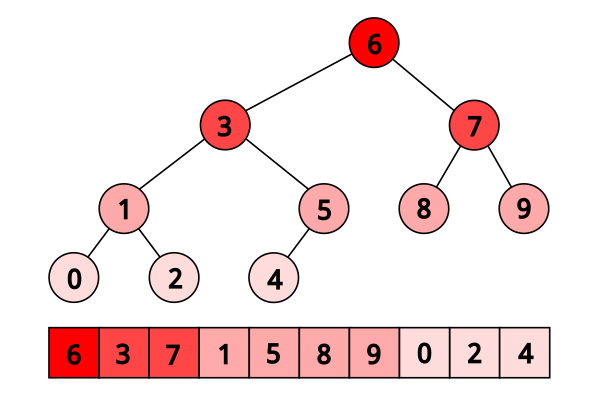
Figure 1: A picture of the Eytzinger layout (taken from Algorithmica)
As for how to build the layout from a sorted array, there is a simple recursive algorithm which is well described in Algorithmica, so we will not waste space here and will refer the reader there if interested.
So, why should Eytzinger be better? The whole problem of array searching is memory bound; it is about how how many levels of the search can we fit into caches so that we don’t have to do many main memory requests. Using this lense, in many ways, a normal sorted array and Eytzinger are similar. Eytzinger is very efficient at caching values at the top of the tree (one fetched cacheline of 64B contains 4 layers there) while sorted array is efficient in the same manner at the bottom of the tree. In addition, Eytzinger will allow us to more efficiently prefetch all the possible paths up to 4 steps into the future.
Algorithmica finds that in the end, it is the efficient prefetching that leads to good performance. For us, when conducting many queries, caching the top should also be better, because it can be better reused and leads to less main memory traffic overall. We shall see whether that holds up.
3.1 Naive implementation Link to heading
The API stays the same as for normal binary search; we get a query and
we return the lower bound or u32::MAX when the lower bound does not
exist.
Notice that indexing starts from one. This makes the layout a bit easier to implement, is a bit more pleasant to caches (layers of the tree will be aligned to multiples of cache size), and allows us to easily handle the case where the lower bound does not exist, as the way we calculate the final index will result in zero.
| |
When you think about it, you see that the first while loop looks through the array, but the index it generates in the end will be out of bounds. How do we then get the index of the lower bound?
I needed some time to grok this from the Algorithmica post, so I will
write it here in my own words. Essentially, each iteration of the
while loop resembles either going to the left or to the right in the
binary tree represented by the layout. By the end of the loop, the index
will resemble our trajectory through the tree in a bitwise format; each
bit will represent whether we went right (1) or left (0) in the tree,
with the most significant bit representing the decision on the top of
the tree.
Now, let’s think about how the trajectory finding the lower bound will
look. Either we will not find it, so the trajectory will be all ones,
since q was always greater than each element of the array. Then we want
to return the default value, which we have stored at index 0 of the
self.vals array.
In the case the lower bound was found, we infer that we compared q
against it once in the trajectory, went left and then only went right
afterwards (because it is the smallest value >= q, all values smaller
than it are smaller than q). Therefore, we have to strip all the right
turns (ones) at the end of the trajectory and then one bit.
Putting this together, what we want to do is this (hidden in the function
search_result_to_index):
| |
Okay, let us see how it performs!

Okay, so we see the layout is a bit slower at the smaller sizes and not too great at the large array sizes. So far, not too good. Notice the bumps; we have already seem those when looking at the naive implementation of binary search. These are also caused by the branch predictor not knowing when to stop the loop. We will deal with them later.
3.2 Prefetching Link to heading
The great thing about Eytzinger is that prefetching can be super effective. This is due to the fact that if we are at index \(i\), the next index is going to be at \(2i\) or \(2i + 1\). That means that if we prefetch and the subsequent values are well aligned inside a single cache line (which they will be), we can actually prefetch both of the possible options at once!
We can make use of this effect up to the effective cache line size. A usual cache line size
is 64 bytes, meaning that the cache line can fit 16 u32 values.
If we prefetch 4 Eytzinger iterations ahead, e.g. to position \(16i\),
we can get all the possible options at that search level in a single
cache line! So, let’s implement this:
| |
As for the performance, it gets a lot better at large sizes:

And we can see that prefetching 4 iterations ahead is really best, which makes sense, because we’re not really doing more work, we’re just utilizing the fetched cachelines better.
3.3 Branchless Eytzinger Link to heading
Now, we will fix the bumpiness in the Eytzinger graph. This is caused by branch mispredictions when deciding whether to end the loop; if the array size is close to a power of two, the ending is easy to predict, but otherwise, it is difficult for the CPU to see whether to do one more iteration or not. We proceed as Algorithmica suggests, doing a fixed number of iterations and then doing one conditional move if still needed. We also still do prefetching:
| |
As num_iters, we pre-compute the integer logarithm of the size of the array.
The get_next_index_branchless uses an explicit cmov from the
cmov crate. Without it, it was surprisingly difficult to get the compiler to
accept this optimization, as select_unpredictable did not quite work.

On the performance plot, we see that this helps remove the bumps, while costing us a bit of runtime at large array sizes.
3.4 Batched Eytzinger Link to heading
Now, let us do batching the same way we did with binary search. We will consider two variants, prefetched and non-prefetched. The prefetching shouldn’t really be needed; the batching should properly overlay memory requests anyway. But modern computers are strange beasts and we saw prefetching being helpful with batched binary search already, so we’ll try it and we’ll see. See the source code below.
3.4.1 Non-prefetched Link to heading
| |

Without prefetching, we see gains up until batch size 128. We therefore use that as our baseline for further comparisons.
3.4.2 Prefetched Link to heading
| |

With prefetching, batch size of 16 is suprisingly better than larger batch sizes.
We compare the two graphs and compare the two best options, one from prefetched and non-prefetched:

We see that the non-prefetched version with a large batch size is a few percent faster, most likely due to utilizing the memory throughput better. Therefore, we select it as our best eytzinger version.
4 Eytzinger or BinSearch? Link to heading
Now, to compare batched Eytzinger to batched binary search:

We see that Eytzinger is quite a lot faster for both large and small sizes. The reason for this is that Eytzinger is a lot more cache-efficient. To investigate this further, I wrote a small Python script simulating the behaviour of both algorithms with respect to caches.
The setup was a single-layer, fixed-size, direct-mapped cache. What I found was that when it comes to memory throughput, batched Eytzinger is more advantageous. This is because the more-accessed top levels of the tree are more efficiently cached and can be reused between queries. This leads to less cache lines fetched from main memory overall compared to binary search.
So, we have come quite a long way, from one query taking roughly 1100ns to just about 100ns a query on a 1GB array. That is a speedup of 12x, and it was essentially for free! Next, let us look at the multithreaded case where we run the search on many cores.
5 Memory efficiency – parallel search and comparison to S-trees Link to heading
Now let us push memory throughput to its limits and compare the layouts when we are allowed to use multiple threads to query. Keep in mind that when multithreading gets involved, the results are going to be much more noisy; the spreads in the graphs reflect that.
The first interesting aspect of this is whether prefetching will help for Eytzinger or binary search. Let’s first look at binary search:

In the same way as in the single-threaded version, we see that the prefetching helps a bit, as it does not actually add memory traffic, it only hints to the CPU where to look. In the next plot we see that batching is helpful up to roughly size 32, and then it levels out.

We will therefore use batch size 32 as a reference for further comparisons.
As far as Eytzinger goes:
 Here we see that prefetching does not make a big difference. We keep it for the comparison.
Here we see that increasing batch size too much hurts performance on small array sizes, and does not improve performance much beyond batch size 16 on large array sizes. We therefore use batch size 16 as a reference for Eytzinger. So for the final comparison:

In the plot, we also include one of the fast S-tree versions coded by Ragnar to have a direct comparison on my machine. We can see that due to the use of SIMD and better use of caches, S-trees are still much much faster than either Eytzinger or binary search. This is to be expected, because S-trees can do essentially four layers of the search in a single iteration using one memory query whereas binary search or Eytzinger will need four memory requests.
To get this performance, it is crucial that you compile with -C target-cpu=native. I found out the hard way; I forgot to turn this option on in some of my tests and S-trees turned out to be much slower
due to more non-vectorized comparisons compared to both binary search and Eytzinger. I wasted quite some time trying to figure out why that was.
We also see that Eytzinger and binsearch are almost equal; Eytzinger is better at the top while binary search is better at the bottom of the search, and these advantages are rougly of equal value in the multithreaded setting.
We can also look at a direct comparison of single and multi-threaded variants:

Overall, the speedup was roughly 4 (at array size 1GB) when using 8 threads. This clearly indicates that we’re memory bound. If we wanted to go for more speed and more cache utilization, we could start the first \(\lg(n)/2\) layers with the Eytzinger layout and the bottom \(\lg(n)/2\) layers with a standard sorted array. However, we won’t delve into this here, as there is more efficient stuff one can do; check out Ragnar’s post on S-trees! Otherwise, if you are curious, the array layouts paper goes quite in-depth on this.
6 Interpolation search Link to heading
In the static search tree post, Ragnar suggested looking at interpolation search as an option to reduce the amount of accesses to main memory. For completeness, we will implement it here as well to check out how it performs.
The idea behind interpolation search based on the fact if data is drawn from a random uniform distribution, then when we sort it and plot the indices on the x-axis and values on the y-axis, we should roughly get a linear function. Using that, when we have the query and the values at the start and end of the array, we can efficiently interpolate (“guess”) where values corresponding to the query should be. We can iterate this approach, building a search algorithm out of it.
When the input data is nicely evenly distributed, the complexity is \(O(\lg \lg n)\) iterations, rather than \(O(\lg n)\) for binary search. When the data is not well distributed, the worst case complexity is \(O(n)\), which is illustrated by the following example. Imagine we’re searching for 2 in the following array of 10000 elements:
| |
Every time we do the interpolation, we suspect that the 2 is on the second position of the array. Therefore, we reduce the searched area only by one element in every iteration and end up with a linear time complexity.
Even in non-adversarial settings, like with the human genome, we could get into trouble with non-uniform distribution of input data. But let’s try it out anyway and see how it goes.
| |
For the following plots, please notice that compared to the previous section, the scale changed quite drastically, as the results are quite a bit worse for the algorithm.

We see that the performance is mostly terrible, multiple times slower than even standard library binary search, even though it beats it at large array sizes. Looking at perf outputs,
we see that the issue is two-fold. Firstly, there is a data hazard on the if condition in each iteration. But secondly, integer division
is just very slow.
We can see if batching can hide some of this, as it did before:
| |

The performance improves a bit and is decent for large array sizes, but still nowhere close to the level of performance of previous schemes like Eytzinger. The division is a bottleneck and it is hard to optimize it away. I tried to go around it with SIMD, but there, efficient integer division instructions don’t really exist either, and the performance gains are minimal.2
An interesting factor for interpolation search is also how it performs well on non-random data. Therefore, we download a part of the human genome from here and compute 32-bit prefixes of all the suffixes. We then search in a subset of them and measure performance. This should be slower, as the data is not going to be exactly uniformly distributed.
I tried at first with just taking the first X 16-mers, sorting them and then conducting a search on them. I ended up with a really strange result where the time per query would at first increase sharply, then fall and then take off again. The reason for this strange result is that the human data is strongly non-uniform. As interpolation search performs badly with increasing non-uniformity, we can assume that the start of the genome is really, really badly distributed and the distribution goes back to something resembling a uniform one as we increase the size of the sample we’re searching.
I fixed this by not always starting from the beginning, but taking a random starting index in the unsorted array of 16-mers and taking a continuous segment from it. That way, the results will be quite realistic (it makes sense to search through a continuous segment of the genome) but we will avoid the skewed start.

We see that the result is noisy, but more as expected. The results are not really too bad; the data seems to be “random enough”. But overall, it isn’t really enough to make the scheme worthwhile against the other ones. We can see the comparison to Eytzinger in the plot. For completeness we also show the graph for the multithreaded case:

Overall, I did not see this as a priority and did not spend too much time at optimizing it, as it seems like a bit of a dead end. I would appreciate ideas; if you have them, please let me know.
7 Conclusion and takeaways Link to heading
Overall, we found that the conclusions from the Algorithmica article and from the array layouts paper mostly hold even for batched settings. Eytzinger is the best choice for a simple algorithm that is also very fast. It beats standard binary search due to its better cache use characteristics and ease of prefetching. The other major takeaway is of course that batching is essentially free performance and if you can, you should always do it.
For interpolation search, I do not believe the scheme to be too worthwhile; it is difficult to optimize and relies on the characteristics of the data for performance. Given there are schemes like Eytzinger or S-trees that are well suited for modern hardware optimizations, I think you should mostly use those even though the asymptotics are worse.
When writing this, I was suprised to see that the Rust standard library has some optimizations for binary search already implemented, but not all that are recommended by our sources, namely, prefetching is missing. This is suprising, because prefetching arguably does not cost us much anything. Is it due to unavailability of prefetch instructions on some platforms? If you know, I’d be glad if you let me know.
Anyway, it was a lot of fun to go a bit into the world of performance engineering. Thanks to Ragnar for the idea & the opportunity!
Here’s Linus talking about it ↩︎
When reimplementing the batched version with SIMD, I burned myself by thinking that the Rust portable SIMD
clamp()function would do an element-wise clamp. Watch out, it doesn’t, at least not at this time. ↩︎