These are some notes about the Burrows-Wheeler Transform (BWT), FM-index, and variants.
See my post on the linear time suffix array construction algorithm for notation and terminology.
- At the bottom you can find a visualization.
- This page has an interactive demo.
Source code for visualizations is this GitHub repo.
Burrows-Wheeler Transformation (BWT) Link to heading
The BWT of a string \(S\) is generated as follows:
- Generate all rotations of \(S\).
- Sort the rotations. Their order is given by the suffix array of $S$$.
- Store the last column \(L\) of the sorted rotations.
Using the last-to-first mapping described below, the original string can be
reconstructed from this last column! One benefit of applying the BWT to a string
is that typically the BWT contains long runs of equal characters, and hence can
be compressed better. E.g. when a string contains many copies of ABC,
the rotations starting with BC are close together, and many of those will have
an A in the last column.
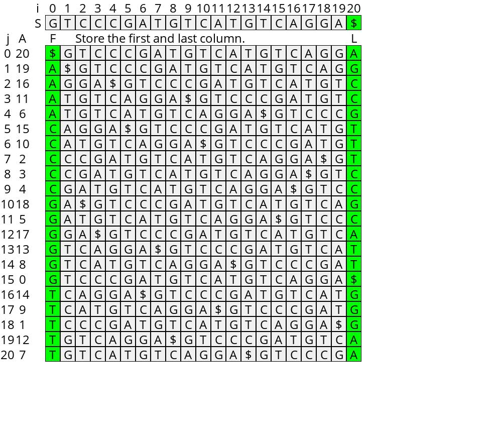
Figure 1: The BWT of a string.
Last-to-first mapping (LF mapping) Link to heading
Now assume that \(S\) ends with a sentinel $.
Look at Figure 2 below, and in particular at those rotations starting with G. Since
all those rotations start with the same character, dropping this first character
from each of them does not change their relative order. In fact, these are
rotations, so this is equivalent to rotating the string by one, moving the first
character to the back. Thus, the order of G’s in the last column is the same as
in the first column.
![Figure 2: The LF correspondence: the order of the rotations starting with G is the same as those ending with G. The j=14’th sorted rotation (the 5’th starting with a G) starts at index i=8. The next character is a T at position i=9. The suffix-array entry for this T (j=17, A[17]=9) is the 5’th rotation ending in G.](/ox-hugo/lf.png)
Figure 2: The LF correspondence: the order of the rotations starting with G is the same as those ending with G. The j=14’th sorted rotation (the 5’th starting with a G) starts at index i=8. The next character is a T at position i=9. The suffix-array entry for this T (j=17, A[17]=9) is the 5’th rotation ending in G.
Now, we define the LF-mapping as follows: Given a position \(j\) in the suffix array, the LF-mapping of \(j\) is the position in the suffix array of \(A[j]-1\), i.e., the sorted position of the previous-suffix of the \(j\)’th row.
To efficiently compute this, we use two datastructures, shown in Figure 3:
- \(C[c]\) counts the number of characters less than \(c\) in \(S\).
- \(Occ[c][j]\) counts for each character \(c\) and each BWT-index \(j\) the number of rotations ending in \(c\) before position \(j\).
Now, suppose that rotation \(j\) that starts at \(i:=A[j]\) in the string \(S\) ends in character \(c:=s_{i-1}\). Then, \(S_{i-1}\), the suffix starting at position \(i-1\), starts with a \(c\) and is followed by \(S_i\). We can find its position in \(A\) as follows:
- There are \(C[c]\) entries with a character \(<c\) that we must skip first, since \(S_{i-1}\) starts with a \(c\).
- Then, because of the LF-correspondence, the number of entries starting with \(c\) that must be skipped is the same as the number of \(c\)’s in the last column before position \(j\), i.e. \(Occ[c][j]\).
- Thus, \(LF(j) = C[c] + Occ[c][j]\), or equivalently, \(A[C[c] + Occ[c][j]] = j-1\).
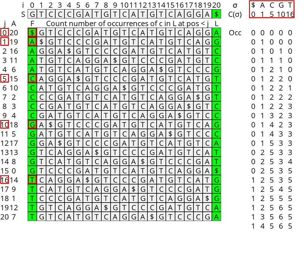
Figure 3: The LF Mapping datastructures Occ counting the number occurrences of each character before each position, and C, the number of characters less than each character.
Pattern matching Link to heading
Now suppose we would like to find the range of the suffix array that starts with some pattern/query \(Q\). It turns out the LF mapping can help us to answer this in \(O(|Q|)\) time. The idea is to start at the end of the query and iteratively prepend characters, while keeping track of the range of the suffix array that corresponds to the current suffix of the query.
The core observation is this: Let \(s_i\) be the first position in the suffix array starting with the query-suffix \(Q_i = q_i \dots q_{|q|-1}\). (Or more generally, the first position \(j\) with \(S_{A[j]} \geq Q_i\).) Then, if we prepend character \(c:= q_{i-1}\), exactly the first \(Occ[c][s_i]\) rotations starting with \(c\) will be less than \(Q_{i-1}\). Thus, the new starting position of the range is
\begin{equation} s_{i-1} = C[q_{i-1}] + Occ[q_{i-1}][s_i]. \end{equation}
Similarly, we can define the (exclusive) end \(t_i\) of the range as the first index starting with a string \(>Q_i\). We update it using the same rule:
\begin{equation} t_{i-1} = C[q_{i-1}] + Occ[q_{i-1}][t_i]. \end{equation}
The initialization is for \(i=|Q|\) where the corresponding interval is the entire suffix array: \(s_{|Q|} = 0\) and \(t_{|Q|} = n\).
Note that when no rotation starting with \(Q_i\) ends in \(q_{i-1}\), i.e. when \(Occ[q_{i-1}][s_i] = Occ[q_{i-1}][t_i]\), the values of \(s_{i-1}\) and \(t_{i-1}\) become equal. This means that the search range is empty and \(Q_{i-1}\) does not occur in the string. In this case, \(s_i\) and \(t_i\) still indicate the position where the query suffix would be ordered in the suffix array.
One step of this process is shown in Table 1 and fully in the visualization at the end.
CC) have been processed to give the range from s_2=7 and t_2=9. The next character is c=s_1=T. There are C[T]=16 characters <T, 2 T's before the start of the interval, and 3 T's before the end of the interval. Thus, the new interval (shown on the right) is from s_1=16+2=18 to t_1=16+3=19.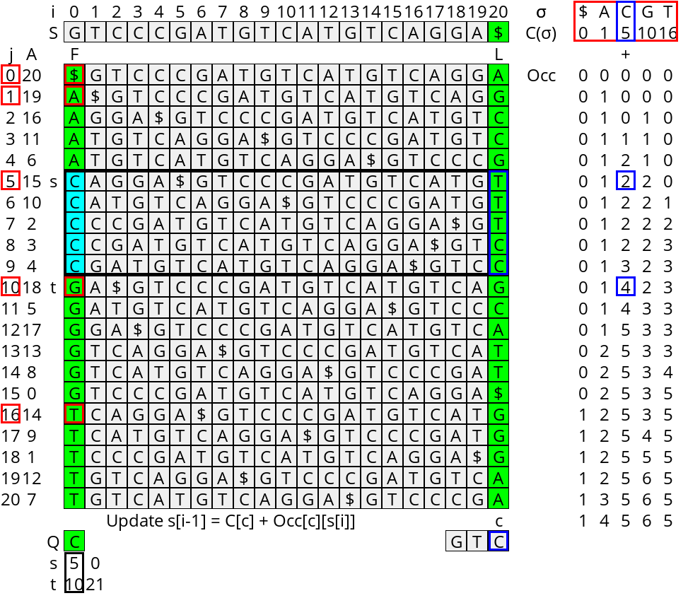 | 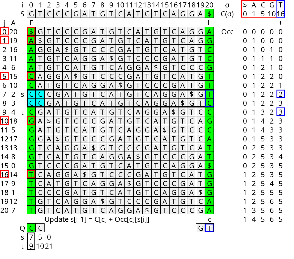 |
Visualization Link to heading
This visualization is generated using the code here. If you run that yourself you can use any input and query string and step through at your own pace.
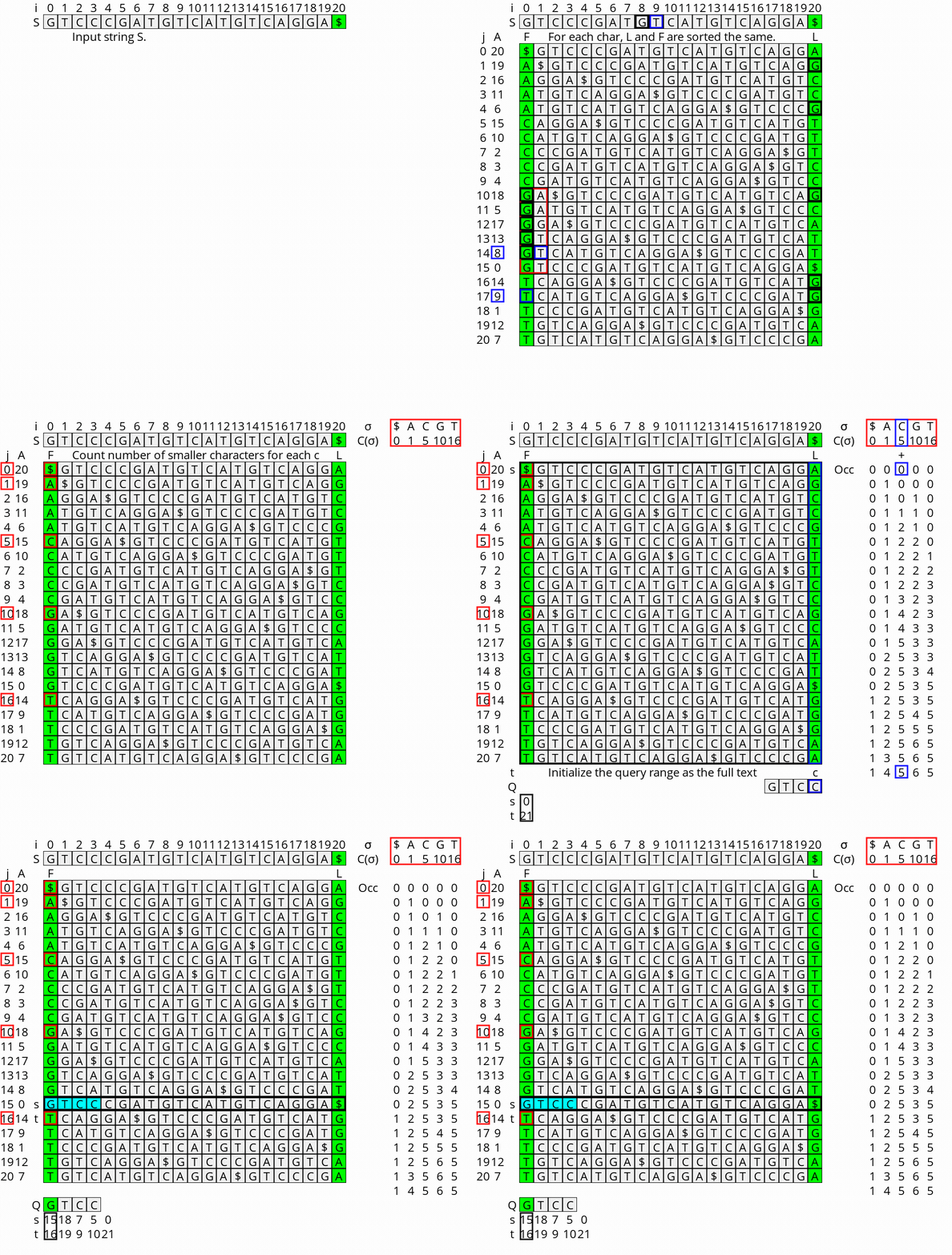
Figure 4: Visualization of the construction of the BWT, FM-index, and how they can be used to query a string.
Bi-directional BWT Link to heading
Using the method above we can find the SA-range after prepending characters to a query. It would be cool if we could also extend the query on the right.
Since the strings starting with \(Qc\) all start with \(Q\), the SA-range \([s’, t’)\) for \(Qc\) is a subset of the range \([s, t)\) for \(Q\). To find the exact range, we must determine the number \(a\) of times a character \(<c\) occurs after \(Q\). This will give \(s’ = s+a\). The end of the interval is given by the number of times \(b\) a characters \(\leq c\) occurs right after \(Q\): \(t’ = t + b\).
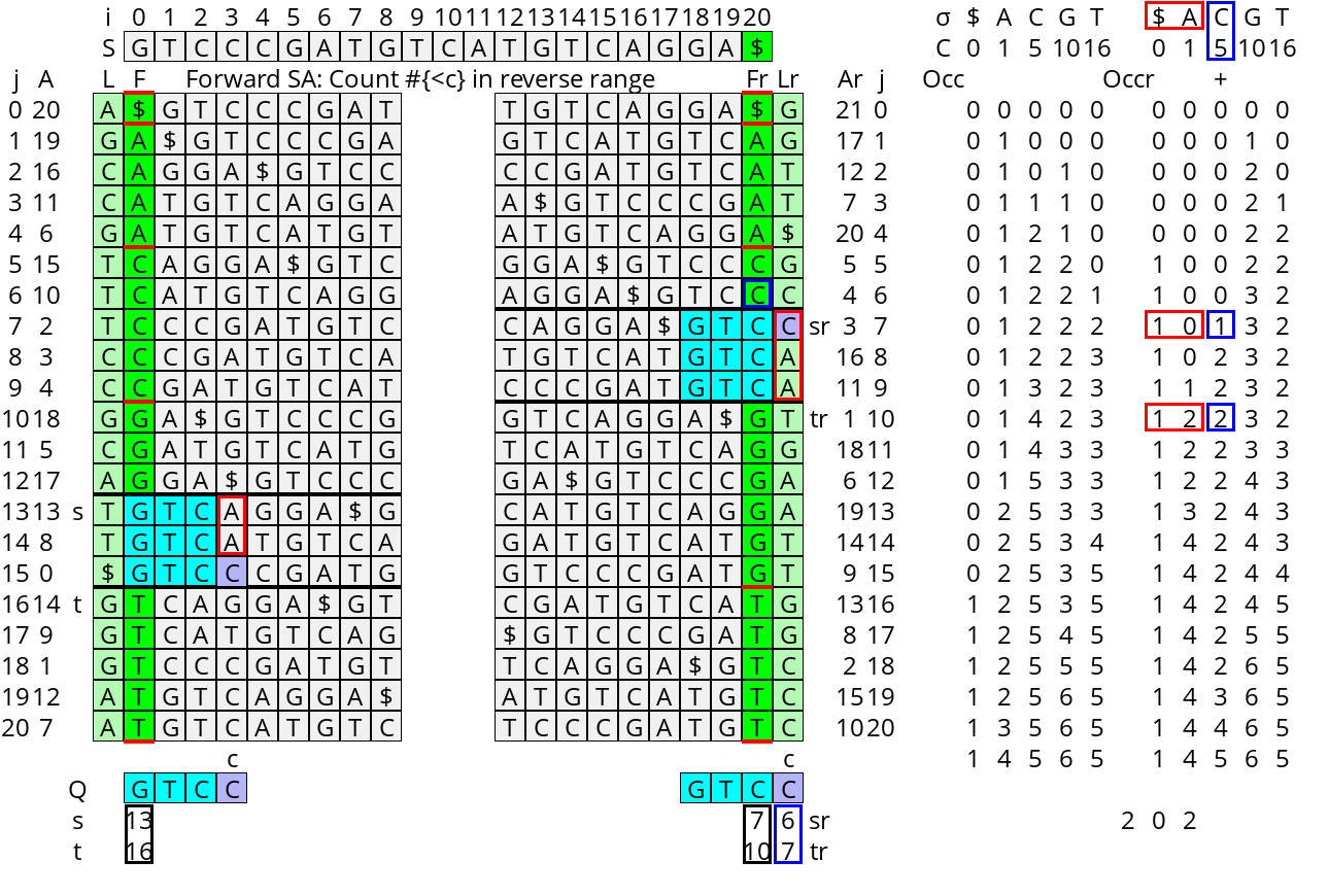
Figure 5: The red boxes indicate that the set of characters following matches (cyan) of Q in the forward suffix array (left) is the same as the set following the matches of Q in the reverse suffix array (right). To count the number of highlighted characters less than c, we can use the occurrences array of the reverse suffix array.
Using an \(Occ\) array for each column it would be easy to answer these queries, but this requires quadratic memory. Instead, note that the \(Occ\) array we already have allows us to count the numbers we need for the last column, i.e. the column before \(Q\). The crucial idea is to use the suffix array of the reverse string \(\overline S\) and track the interval of prefixes \(Q\) in the forward SA and interval of suffixes \(Q\) in the reverse SA in lockstep.
Updating the state: Let \(\overline A\) be the suffix array of the reverse string \(\overline S\) and \(\overline{Occ}\) be the corresponding occurrences counts. The character counts \(\overline C = C\) remain the same. The state of a query is \(([s, t), [\overline s, \overline t))\), an interval of \(A\) and \(\overline A\). This is initialized to \(([0, n), [0, n))\) for the empty query. When appending \(c\), the update for the forward interval becomes
\begin{align} s’ =& s + \sum_{c’ < c} \left(\overline{Occ}[c’][\overline t] - \overline{Occ}[c’][\overline s]\right)\\ t’ =& s + \sum_{c’\leq c}\left(\overline{Occ}[c’][\overline t] - \overline{Occ}[c’][\overline s]\right), \end{align}
while the reverse range is updated as before:
\begin{align} \overline s’ =& C[c] +\overline{Occ}[c][\overline s] \\ \overline t’ =& C[c] +\overline{Occ}[c][\overline t]. \end{align}
Prepending a character \(c\) is the same with the roles of the forward and reverse SA swapped.
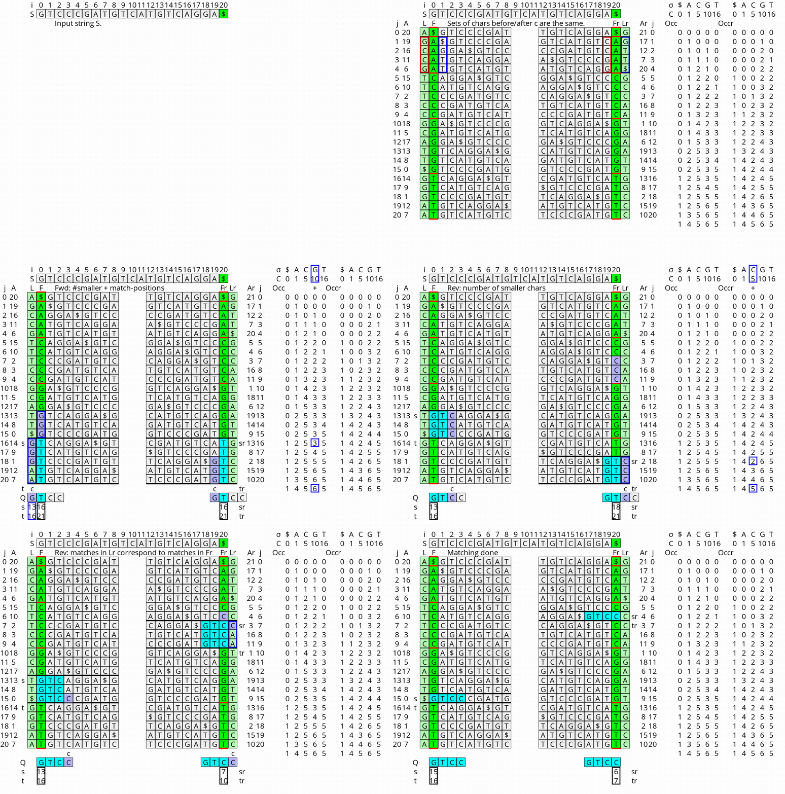
Figure 6: Visualization of the bidirectional BWT and how it can be used to extend queries in two directions.