\[ \newcommand{\inv}{^{-1}} \newcommand{\di}{\delta\inv} \newcommand{\poly}{\mathrm{poly}} \]
This post summarizes some recent results and idea on various types hash tables. Collected together with Stefan Walzer.
- “Iceberg Hashing: Optimizing Many Hash-Table Criteria at Once” (Bender et al. 2023)
- “IcebergHT: High Performance Hash Tables through Stability and Low Associativity” (Pandey et al. 2023)
- “Tight Bounds for Classical Open Addressing” (Bender, Kuszmaul, and Zhou 2024)
- “Optimal Bounds for Open Addressing without Reordering” (Farach-Colton, Krapivin, and Kuszmaul 2024; Farach-Colton, Krapivin, and Kuszmaul 2025)
- “Optimal Non-Oblivious Open Addressing” (Bender, Kuszmaul, and Zhou 2025a, 2025b)
1 Types of hash tables Link to heading
- Open addressing
- Elements are stored in a single (slot) array with no additional metadata.
- Stable
- As soon as an element is inserted, it does not move (apart from resizing).
- Greedy
- When inserting an element, the first empty slot found in the probe sequence is where it will go.
- Oblivious
- The probe sequence for a key \(x\) is \(h_1(x)\), \(h_2(x)\), \(\dots\), without depending on (meta)data in the hash table.
- Dynamic resizing
- The load factor is high at every point in time.
- Fixed-capacity
- The opposite of dynamic resizing, when the table is always near-full.
- Independent hash functions
- Some hash tables require fully random hash functions, while for others, $O(1)$-independence is enough.
2 Metrics Link to heading
- Universe size \(u\)
- Keys are chosen in \(0\leq k < u\). We may use \(w := \lg u = \lg_2 u\).
- Hash table size \(n\)
- The hash table contains \(n\) slots.
- Elements \(k\)
- We have \(k\) distinct keys.
- Load factor
- \(k/n = 1-\delta\) of the slots are filled. Also \(1-\varepsilon\) is used. I’ll call \(\delta=\varepsilon\) the slack or overhead, but neither seems standardized.
Generally, the goal of this line of research is to make dense hash tables with overhead as close to 0 as possible.
We can then measure query, insertion, and deleting time (together called operations). Almost always, an expectation over the random hashes is taken. Then, one can consider e.g. (from strong to weak):
- Constant time operations, with high probability1, and so this implies constant time in expectation.
- \(O(1)\) worst case expected time.
- \(O(1)\) amortized expected time.
3 Lower bounds Link to heading
- Static set
- The entropy of choosing \(n\) elements2 of \(u\) is \[\lg \binom un \approx n \lg u - n \lg n,\] ans this is a lower bound on the size of a hash table. In particular, this is less than the \(n \lg u\) bits needed to list the keys.
4 Iceberg hashing (2023) Link to heading
See Bender et al. (2023)
- \(\delta = o(1)\)
- stable, apart from resizing
- (Either resize in bulk, or de-amortize and be unstable for a while.)
- \(\lg \binom un + n \lg lg n\) space, which is optimal
- dynamic resizing
- \(O(1)\) queries whp
- \(1+o(1)\) cache misses
5 IcebergHT (2023) Link to heading
See Pandey et al. (2023)
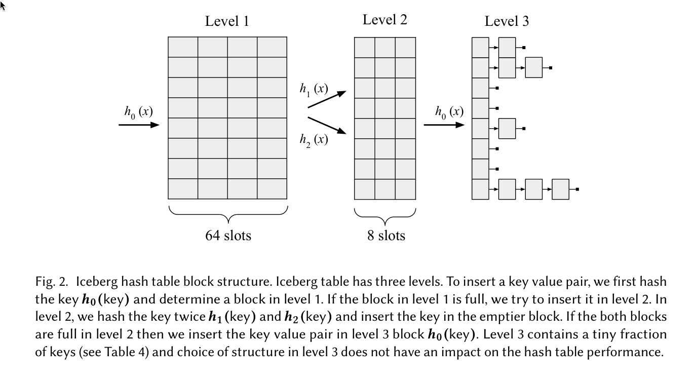
Figure 1: Screenshot from Pandey et al. (2023).
6 Tight Bounds for Classical Open Addressing (2024) Link to heading
See Bender, Kuszmaul, and Zhou (2024).
Introduces rainbow hashing:
- \(O(1)\) expected-time queries,
- \(O(\lg \lg \di)\) expected-time insertions and deletions, and this is optimal.
- Also supports dynamic resizing, with no further cost.
- First work to have \(o(\di)\) complexity for all of insertion, deletion, and queries simultanuously.
7 Optimal Non-oblivious Open Addressing (2025) Link to heading
See Bender, Kuszmaul, and Zhou (2025b).
- \(\delta=0\), ie completely full table.
- Dynamic resizing.
- \(O(1)\) hash functions that are $O(1)$-wise independent.
Non-oblivious: information is stored in the order of the keys, and this is used to speed up probing. But how exactly?
Where there are \(n\) elements in an array, their order encodes \(\log n! = \Theta(n \log n)\) bits of information that we could exploit.
Universe reduction: if \(u = \Omega(\poly(n))\), when we can (whp) use a random hash function to injectively map all keys into a smaller universe of size \(u’ = \poly(n)\).
Partner hashing: This is the crux to using the stored elements. We can put a different element \(y\) in the preferred location of a key \(x\), and then \(x\) gets send to \(y\)’s location. But I haven’t fully understood the details yet.
8 Optimal Bounds for Open Addressing Without Reordering Link to heading
See also this earlier post.
8.1 Funnel hashing Link to heading
See (Farach-Colton, Krapivin, and Kuszmaul 2024).
- \(O(1)\) amortized probe complexity
- \(O(\log^2 \di)\) worst-case expected queries
- \(O(\log \di)\) (worst-case?) insertions?
8.2 Elastic hashing Link to heading
- \(O(1)\) amortized probe complexity
- \(O(\log \di)\) worst-case expected queries
- \(O(\log \di)\) (worst-case?) insertions?
References Link to heading
W.h.p. means with probability \(1-O(1/n^c)\) for every \(c>0\), assuming data-structure constants are suitably chosen dependent on \(c\). ↩︎
It’s a bit confusing that we have \(k\) keys in \(n\) slots but use \(n\) in such formulas. But since the load factor is close to \(1\), it doesn’t really matter. ↩︎