- 1 Construction of k-PHF using modified PtrHash
- 2 k-PHF Lower bounds
- 3 Cache-optimal k-PHF
- 4 RecSplit
- 5 What is the optimal bin-size distribution for PtrHash-based k-PHF
- 6 Halfway bin-size for \(k=2\)
- 6.1 First half
- 6.2 Second half
- 6.3 Total
- 6.4 First-half optimum
- 7 Optimal bin-size distribution
- 8 Optimal choice of seed
- 8.1 Non-minimal case
- 9 Practical idea?
- 10 Lower bound proofs
There are ongoing notes on lower and upper bounds for non-minimal k-perfect hashing based on discussions with Stefan Walzer, Stafan Hermann, and Peter Sanders.
1 Construction of k-PHF using modified PtrHash Link to heading
Code at src/kphf.rs at http://github.com/RagnarGrootKoerkamp/static-hash-sets
slot_ratio: number of slots to use relative to \(n\).meta_ratio: size of metadata relative to total input size.sort: sort the buckets by size or not?
Results for \(k=16\):
| |
Conclusion: we can construct k-PHF with 20% extra slots and 0.1% relative size of the metadata.
Thus, for \(\alpha=1/1.2 = 0.83\), we can get 0.064 bits/key. Pushing it a bit more, with meta_ratio down to 0.00085 we get 0.0544 bits/key when using consensus. I can now not reproduce the 0.0320 bits/key bottom rows of the table anymore.
The corresponding lower bound (see script below) is 0.0362, which indeed is above the 0.0320.
2 k-PHF Lower bounds Link to heading
For minimal k-PHF, the brute-force solution admits \(\binom{n}{k,\dots,k}\) solutions, so needs \((n/k)^n / \binom{n}{k,\dots,k}\) tries, which corresponds to \(\log e + \log((k!)^{1/k} / k)\) bits.
For load factor \(\alpha\), this script computes the lower bound for non-minimal $k$-PHF.
| load \(\alpha\) | k=1 | k=2 | k=4 | k=8 | k=16 | k=32 | k=64 | k=128 |
|---|---|---|---|---|---|---|---|---|
| 0.1 | 0.07466 | 0.00849 | 0.00022 | 0.0000003 | 0.000000000001 | |||
| 0.2 | 0.15498 | 0.03112 | 0.00259 | 0.00004 | 0.00000002 | 0.00000000000002 | ||
| 0.3 | 0.24202 | 0.06581 | 0.00989 | 0.00052 | 0.000003 | 0.0000000004 | ||
| 0.4 | 0.33724 | 0.11221 | 0.02444 | 0.00267 | 0.00008 | 0.0000002 | 0.000000000003 | |
| 0.5 | 0.44269 | 0.17114 | 0.04833 | 0.00857 | 0.00068 | 0.000012 | 0.000000009 | 0.00000000000001 |
| 0.6 | 0.56140 | 0.24472 | 0.08410 | 0.02095 | 0.00318 | 0.00020 | 0.000002 | 0.0000000006 |
| 0.7 | 0.69828 | 0.33704 | 0.13568 | 0.04360 | 0.01028 | 0.00149 | 0.00009 | 0.0000009 |
| 0.8 | 0.86221 | 0.45624 | 0.21044 | 0.08294 | 0.02699 | 0.00677 | 0.00113 | 0.00009 |
| 0.9 | 1.07359 | 0.62179 | 0.32631 | 0.15418 | 0.06498 | 0.02404 | 0.00755 | 0.00188 |
| 0.95 | 1.21522 | 0.73972 | 0.41651 | 0.21663 | 0.10374 | 0.04552 | 0.01815 | 0.00647 |
| 0.98 | 1.32751 | 0.83742 | 0.49629 | 0.27699 | 0.14560 | 0.07194 | 0.03332 | 0.01444 |
| 0.99 | 1.37558 | 0.88056 | 0.53318 | 0.30680 | 0.16811 | 0.08765 | 0.04339 | 0.02036 |
| 0.999 | 1.43271 | 0.93321 | 0.58010 | 0.34702 | 0.20111 | 0.11335 | 0.06222 | 0.02895 |
| 1.0 | 1.44269 | 0.94265 | 0.58893 | 0.35509 | 0.20832 | 0.11967 | 0.06761 | 0.03770 |
2.1 Estimated lower bounds for variants Link to heading
\(k=8\):
- regular: 0.36
- windowed: 0.08
- 4-aligned: 0.13
\(k=16\):
- regular: 0.21
- windowed: 0.02
- 4-aligned: 0.05
3 Cache-optimal k-PHF Link to heading
Given \(n\), \(k\), and \(\alpha\), one can optimize two different things:
- The overall size of the MPHF
- The number of queries answered by a fixed-size cache.
These are different! For eg bucket-placement techniques, you want to balance the size of the bins as much as possible to ensure there are sufficient empty bins until the end. Whereas in order to answer as many keys as possible using the cache, you would rather have a very unbalanced bin size distribution and then use more space afterwards to work around this.
4 RecSplit Link to heading
RecSplit takes the keys and repeatedly splits it into parts until only parts of size (at most) \(k\) remain. The original RecSplit already provides a minimal k-PHF when \(k\) is a power of \(2\). It has \(O(1)\) overhead per split when each split is encoded independently, and smaller overhead when consensus is used. Note that the shape of the splitting tree does not matter: it can be either ‘repeatedly split off the bottom \(k\)’ or repeatedly ‘split in half’.
Strategies for splitting off the bottom \(k\):
4.1 Accept \(\leq k\) Link to heading
Choose a \(\lambda\). Then hash all keys and accept each with probability \(\lambda / n\). Accept the bin when the size \(\mathrm{Po}(\lambda) \leq k\). Choose \(\lambda\) such that the expected size of the truncated distribution equals the average load \[\mathbb E[\mathrm{Po}(\lambda)_{\leq k}] = \alpha k.\] The problem is that this needs many tries when \(\alpha \to 1\).
Instead, do the following: accept the bin only when it has size between \(k-x\) and \(k\) inclusive, for some integer \(x\) depending on \(\lambda\) such that the expected size is (roughly) \(\alpha\). To make this work exactly, accept \(k-x\) itself only with some probability. Then choose \(\lambda\) such that the probability of accepting the bin is maximized.
This script does something similar, but only considers a ‘backlog’ of previously unplaced keys for each bin, rather than all keys. It gets reasonably close (within 30% or so) of the lower bound:
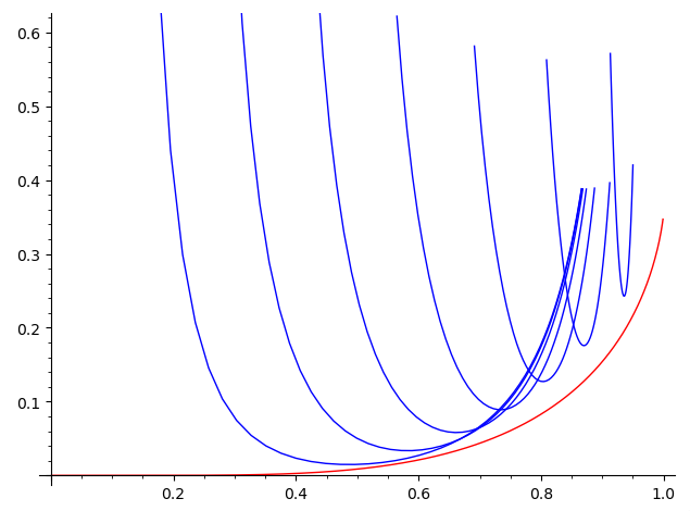
Figure 1: red: space usage of $α$-PHF for (k=8). Blue: space usage of the greedy ‘backlog’ strategy for various parameters.
With consensus, this should also have quite small overhead.
5 What is the optimal bin-size distribution for PtrHash-based k-PHF Link to heading
At the end, the bins follow some size distribution. When bruteforcing a seed, this is simply a truncated Poisson distribution with expected value \(\alpha k\).
When choosing a seed, we should choose the one that makes the distribution most /flat//uniform, with respect to some metric.
We considered the case \(k=2\) and the optimal distribution of bin-sizes after half the keys have been places. When halfway through all bins have size \(1\), we basically build two MPHFs on \(n/2\) keys, for 1.4 bits/key overall.
When halfway through half the buckets have 2 keys, we sort-of build a $k=2$-MPHF on the first and second half of keys. For the first half we select \(n/2\) ‘random’ buckets which saves \(n/2\) bits, but then pay \(n/2\) bits to actualy map into them. (Thus, building a $2$-MPHF on \(n/4\) bins is exactly as hard as building a $2$-PHF with bins of size \(0\) or \(2\) on \(n/2\) bins.) The second half of keys needs \(n/2\) extra bits to map into the gaps left behind by the first half. In the end, this uses 1.4 bits/key as well.
So, the optimal choice must be to have somewhere between \(0\) and \(n\) bins of size \(1\) halfway through.
5.1 Optimal bucket bunction for minimal k-PHF Link to heading
See Hermann et al. (2025):
- github:stefanfred/engineering-k-perfect-hashing/…/OptimalBucketFunction.hpp
- github:stefanfred/engineering-k-perfect-hashing/…/muericalIntegrationBucketFunction.cpp
6 Halfway bin-size for \(k=2\) Link to heading
Suppose we are incrementally building a $2$-MPHF on \(n\) keys. At some point, we have assigned half the keys, and at that point there are \(a\) bins of size 2, \(b\) bins of size 1, and \(c\) bins of size 0, with \(a+b+c=n/2\) (the total number of bins) and \(2a+1b+0c=n/2\) (half the keys). This implies \(a=c=(n/2-b)/2\). Now say we have \(b=\beta n/2\) of the bins with 1 key in them. We want to derive 2 numbers:
- The entropy/bits/space needed to map first half of keys.
- The space needed to map the second half of keys.
and from this we get the space needed for all keys.
6.1 First half Link to heading
We first choose the bins we are going to use: \[A:=\binom{n/2}{a,b,c}\] Then, we choose exactly which keys go into each bin: \[B:=\binom{n/2}{\underbrace{2,\dots, 2}_{a\times}, \underbrace{1,\dots, 1}_{b\times}}\] The total number of functions mapping the first half of keys into the \(n/2\) bins is \[N:=(n/2)^{n/2}.\] We compute the number of bits per element needed to store a suitable function for the first half as \[S_1:=\frac 1n \log \frac{N}{AB} = \frac 12 \log e - \frac 14(1-\beta) - \frac 12 H(\beta)\] where \(H(x) = - x\log(x) - (1-x)\log(1-x)\) is the entropy of \(\beta\).
(Note that I’m normalizing by \(\frac 1n\) here, so this is bits/key over all \(n\) keys.)
6.2 Second half Link to heading
The bins that the keys go to are now fixed. So the number of suitable functions is \[C:=\binom{n/2}{\underbrace{2,\dots, 2}_{c\times}, \underbrace{1,\dots, 1}_{b\times}}\] which equals \(B\) since \(a=c\).
The total number of functions for the second half is again \(N\). We then get \[S_2:=\frac 1n \log \frac{N}{C} = \frac 12 \log e + \frac 14 (1-\beta).\]
6.3 Total Link to heading
The \(\frac 14(1-\beta)\) terms cancel, and the total space is \[S:=S_1+S_2=\log e - \frac 12 H(\beta)\]
Thus, \(\beta=0\) and \(\beta=2\) both require \(\log e\) bits/key, corresponding to our earlier analysis. Optimal is \(\beta=1/2\), ie half the bins having 1 element, where the total space usage is \(\log e - \frac 12\) which indeed is exactly the optimal space usage of a 2-MPHF.
A property of \(\beta=1/2\) is that then, the number of keys in size-1 bins exactly equals the number of keys in size-2 bins. But those do not equal the number of keys in size-0 bins, so this feels slightly ad-hoc I’d say.
6.4 First-half optimum Link to heading
Note that the \(\beta=\frac 12\) that minimizes the overall space is not the same as the one that minimizes the space for the first half. That, instead, is at \(\beta = \sqrt 2 - 1 \approx 0.414\) (wolfram alpha) with value \[S_1(\sqrt 2 - 1) = 0.0855 \textrm{ bits/key}\] whereas with the globally optimal value we have \[S_1(1/2) = \frac 12 \log e -\frac 18 - \frac 12 = 0.0963 \textrm{ bits/key}\] which is slightly more, but not too much.
The total memory in these two cases is: \[S(\sqrt 2-1) = 0.9533\] and \[S(1/2) = 0.9426\]
Summarizing:
| \(\beta\) | \(S_1\) | \(S = S_1+S_2\) |
|---|---|---|
| \(\sqrt 2-1\) | 0.0855 | 0.9533 |
| \(1/2\) | 0.0963 | 0.9426 |
| diff | 0.0108 | -0.0107 |
Curiously, the space we save at the halfway point is (almost?) exactly (up to rounding errors?) the space we then loose overall.
7 Optimal bin-size distribution Link to heading
Based on the above, note that at the halfway point, \(\beta = 1/2\) gives 25% bins of size 0, 50% bins of size 1, and 25% bins of size 2. That is exactly the binomial distribution! Thus, we hypothesize that, if the goal is to reach \(\alpha=1\), at any point in time, the distribution of bin-sizes should follow a binomial distribution.
Equivalently: the probability of putting a key in a bin should scale with the number of empty slots in the bin. (Nice edge case: empty bins then have probability 0.) Or: for each key we choose a random empty slot, rather than a random bin.
Another way of looking at this: if at some point the \(B\) bins have \(s_1, \dots, s_B\) empty slots remaining (for \(S=s_1+\dots+s_B\) remaining keys), the total number of remaining good functions that works is \(G:=\binom{S}{s_1, \dots, s_B}\), out of \(T:=(n/B)^{S}\) functions in total. The number of tries to find a good function is then \[ T/G = \frac{(n/B)^S}{\binom{S}{s_1,\dots, s_B}} = \frac{(n/B)^S}{S!} \prod_i s_i! \] Thus, we want to minimize the cost/ badness \(\prod s_i\).
Specifically, if we have some current badness \(b\) and we have a seed for a bucket with \(\ell\) keys that puts them in (distinct) bins with \(s^1, \dots, s^\ell\) remaining free slots, the badness goes down by \(\prod s^i\), and so we want to choose a seed that maximizes this product.
Unfortunately, using this cost function in my k-PHF variant of PtrHash does not seem to work too well, and it causes more collisions than simply choosing the seed that (lexicographically) minimizes the number of largest buckets it hits.
8 Optimal choice of seed Link to heading
How many bits/key do we need? Then derive bucket function from that.
- Place 1 key at a time.
- Butting it in a bucket with \(s\) empty slots (relatively) reduces the hardness by \(s\times\), when aiming for minimal k-PHF in the end.
- We can spend 1 bit to put a key in a bucket with 2x more empty slots.
- Choose a seed that optimizes
entropy(seed) + entropy(remaining work).entropy(seed)can (hopefully?) be approximated as \(\lg_2 s\)?
- In particular, we would like that
entropy(chosen seeds) + entropy(remaining work)remains roughly constant during construction, as we insert keys one-by-one. For some seeds we’ll be lucky and it goes down, whereas for others we’ll be unlucky and it goes up. - Somehow encode all these seeds efficiently.
- To use consensus we’d need to actually consider multiple tries for each seed, and weigh them relative to each other.
- With bucketing, we group multiple keys together, to hopefully reduce the variance in the size of the seeds.
- Can we compute the expected entropy of the $i$th seed? From that, we can say that we want 8-bit buckets, and then compute the optimal bucket function.
- What about backtracking for bucketed construction?
8.1 Non-minimal case Link to heading
- In the non-minimal case, computing the required entropy is harder, as it requires iterating over all possible distributions of the remaining empty slots. (At least we are not yet aware of an efficient way of doing this.)
- Even worse, after some elements have been placed, we get a matrix of
C[i][j]indicating thatC[i][j]bins are currently filled withikeys and getjempty slots. We have to iterate over all such matrices that sum to the correct total number of (empty) slots.- Then for each matrix we can compute the number of good functions resulting in this matrix, and sum these.
- The entropy is then related to the log of the total number of good functions.
- Maybe a DP can make this efficient in practice? Or maybe we can ignore most terms after showing via tail-bounds that they have negligible contribution to the sum?
9 Practical idea? Link to heading
Inspired by IcebergHT (Pandey et al. 2023), see this post on hash table bounds for a screenshot.
- We make buckets of 64 elements.
- We store a 64-byte (single-cache line) filter for each bucket, containing an 8-bit
fingerprint for each element.
- This allows much larger k than if we store key-value pairs inline directly.
- With 64-bit keys and 64-bit values, we’d pretty much need 2 cache misses anyway?
- Rather than falling back to secondary structures, as in IcebergHT, we put a
64-PHF in front of this. See table at the top for space bounds. At 90% load:
0.0075 bits/elem, or 2MB metadata for a 16GB array of 64bit total key-value pairs.
- As usual when using a bucket function, almost all queries will be answered using a small prefix anyway.
Drawback: 64 8-bit fingerprints has 25% false-positive rate for both positive and negative queries. We could try something like storing the EF encoding of 60 10-bit fingerprints?
- Store 8 bits explicitly
- Store 128bit 01 mask with unary encoding of how often a multiple of 256 is crossed.
Even stronger:
- map 128 keys to a cache line, and store 4-bit fingerprints + another 4 bits using EF.
- Since the keys are sorted by fingerprint, we roughly know where to look, and so we can start probing from the expected location outwards.
10 Lower bound proofs Link to heading
10.1 Proof of 1-PHF worst-case lower bound Link to heading
The current proof of the lower bound on the space of a minimal 1-PHF is as follows:
- Let the universe be \(U\) of size \(u\), and the input be a set of \(n\) keys in \(U\). Assume \(u \gg n^2\), so that \(\binom un \approx u^n\) holds sufficiently well.
- There are \(X=\binom un\) input sets.
- Each seed encodes some function \(f: U \to [n]\). Such a function is good for \(\prod_{i\in [n]} |f^{-1}|(i)\leq (u/n)^n=:Y\) key sets.
- Thus, to cover all \(X\) possible inputs, we need at least \(X/Y\) functions, and thus, there exists an input that requires at least \(\lg (X/Y)\) bits for the seed.
10.2 Proof of 1-PHF expected-case lower bound Link to heading
Note that the conclusion does not say anything about the number of seed bits for a random key set, just on the worst case key set. We’d like to fix this.
- We assume that the key set is a uniform random subset of size \(n\) of \(U\).
- Note that while the set of keys is now random, the function we construct is still deterministic: each seed \(s\) implies a specific function \(f_s: U \to [n]\).
- Each seed \(s\in \mathbb N\) works with some probability \(p_s \leq Y/X\). These probabilities are not independent, and the inputs that a seed works for can overlap.
- For each input, we fix the seed that we assign to it. (Typically the smallest one that works, but we do not require this.)
- Now each seed has some number \(Y_s\leq Y\) of inputs assigned to it, and \(\sum_s Y_s = X\).
- It remains to encode a seed, which is lower bounded by the entropy of the distribution given by \(p_s = Y_s/X\).
- This evaluates to \[E := \sum_s - p_s \lg p_s = \sum_s \frac {Y_s}X \cdot \lg \frac XY \geq \sum_s \frac {Y_S}X \cdot \lg \frac X{Y_S} = \lg \frac XY,\] which is exactly the same as before.
The week part of this proof is step 4. In any setting where there is some deterministic algorithm that assigns a key to an input, this assumption is satisfied. But would we somehow require less space if the construction algorithm is randomized?
How about this modification:
- Run the construction algorithm, which may be randomized, and let \(p^K_s\) be the probability that it outputs seed \(s\) on input \(K\).
- Let \(p_s := \binom un^{-1} \sum_{K\in \binom Un} p^K_s\) be the probability that it outputs seed \(s\) on a random input.
- Then again we have \(p_s \leq Y/X\) and the entropy needed to encode \(s\) is the same as before.
Still it feels like this has a problem: with the randomized construction we are allowed to encode any working seed, and we want to let the entropy-efficient encoding decide on which particular value is stored, rather than the construction algorithm?
10.3 Lower bound for minimal k-PHF Link to heading
For minimal $k$-perfect hashing, the situation is nearly the same. We now have \(B:=n/k\) bins and \(X = B^n\) functions. Otherwise, all that changes is the bound on the number of functions for which a seed \(s\) works. This is again maximized when all parts of \(f^{-1}\) have the same size, and equals \[Y = \binom {u/n}k^B \approx ((u/n)^k/k!)^B = u^n/(n\cdot k!)^B.\] The rest of the analysis is as before.
10.4 Lower bound for non-minimal k-PHF Link to heading
Now, the situation is more complicated. We want to compute the total number of distributions of \(n\) balls into \(B\) bins, where \(kB = n/\alpha > n\) and \(\alpha=1-\varepsilon\) is the load factor.
In (Walzer 2024), it is shown that when throwing balls into bins, conditioning on every bin containing \(\geq d\) balls yields a truncated Poisson distribution for the number of balls in each bin, with \(\lambda\) such that it yields the right expected value. The same argument should directly work for the \(\leq k\) restriction we have here. Note also that the argument is exact, since it is essentially a counting argument.
Thus, we get that the probability that putting \(n\) balls into \(B=(n/\alpha)/k\) bins satisfies the \(\leq k\) load factors is \(\Theta(b^n)\) for some constant \(b\), and by extension, the number of such functions is \(Y=B^n\cdot \Theta(b^n) = \Theta((bB)^n)\).
The rest is as before.