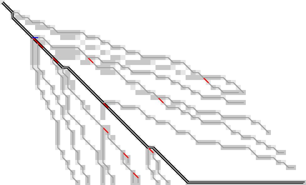
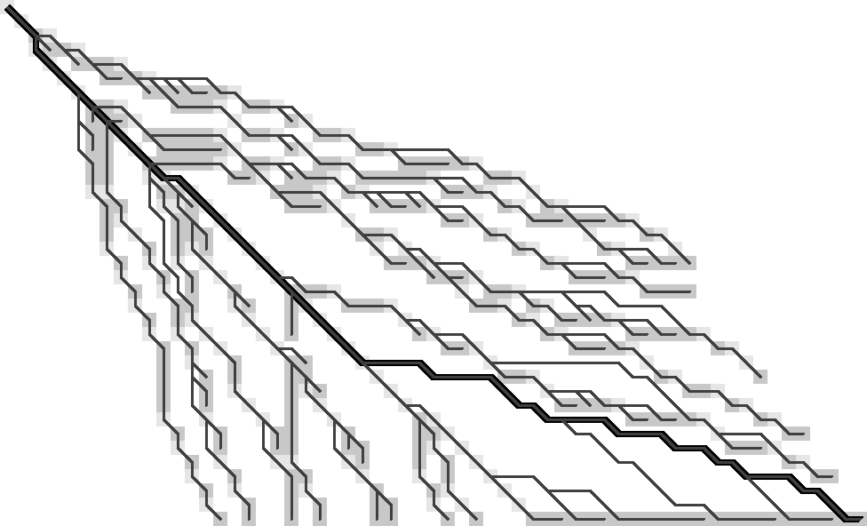
Figure 1: Only the red substitutions and blue indel need to be stored to trace the entire path.
In this post I’ll discuss an idea to run WFA using less memory, while still allowing us to trace back the optimal path from the target state back to the start of the search.
Parts of this were written while I was discovering new things and trying to make this work, so bear with me.
Tl;dr: Storing a small subset of all visited states is sufficient to trace back paths from all furthest reaching points on the active wavefront. For sufficiently nice/simple inputs, this seems to only need \(O(s)\) memory (Figure 1).
Motivation Link to heading
It’s cool! But if you insist (why not simply do BiWFA which does tracing in linear memory?), here’s a post factum argument:
We are also working on A*-based alignment. Meet-in-the-middle for A* is much more complicated than for the simpler Dijkstra and WFA algorithms, and no sufficiently simple bidirectional variant is available to make obvious improvements to A*. Thus, we are stuck with the forward-only version for now. A* already runs smooth on simpler inputs, but needs quadratic memory on bigger/more complicated inputs. Being able to reduce this will hopefully allow better scaling.
Path traceback: two strategies Link to heading

Figure 2: Computing wavefronts step by step in the diagonal-transition algorithm.
First, here is the basic recurrence relation on the furthest reaching (f.r.) points \(f_{s, k}\) (cost \(s\), diagonal \(k\)) for unit-costs (Ukkonen 1985; Myers 1986; Marco-Sola et al. 2021):
\begin{align} f &= \max(f_{s-1, k} + 1, f_{s-1, k-1} +1, f_{s-1, k+1})\\ f_{s, k} &= extend(f). \end{align}
Thus, first we take the maximum furthest-reaching point over the three parents in the current diagonal and the one above/below, and then we extend this point further along matching characters. Figure 2 shows the dependencies between states: columns are diagonals \(k\), rows are wavefronts \(f_{s, \bullet}\), the current cell \(f_{s, k}\) being computed is in green, and its dependencies (the three f.r. points in the maximum) are in dark blue.
The parent f.r. point of a given \(f_{s, k}\) is simply the \(f_{s-1, k’}\) in the arg-max of the maximum. Since we store all previously computed values of \(f_{s,k}\), this is easily computed.
Now, there are two distinct ways to actually recover the path from the parent \(f_{s-1, k’}\) to the current state \(f_{s, k}\):
- Forward greedy
- The first option is the one described in (Marco-Sola et al. 2021): let \(f = \max(f_{s-1, k} + 1,
f_{s-1, k-1} +1, f_{s-1, k+1})\). We have \(f_{s,k} = extend(f) \geq f\), and the
difference \(f_{s,k}-f\) is exactly the number of characters the f.r. point was extended.
To get the path to the parent, we simply walk back \(f_{s,k} - f\) matching characters, and then make a single mutation as needed to get to the parent \(f_{s-1, k’}\).
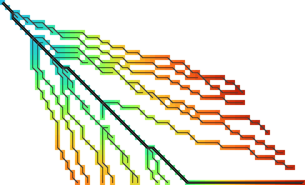
Figure 3: Diagonal transition with forward-greedy path tracing. The coloured cells are the f.r. states computed and stored by diagonal transition. The final path is thick black, and the forward-greedy optimal path to each computed state is shown as thin dark grey lines. Note how paths exactly follow the coloured regions. All figures in this post are generated using this code.
- Backward greedy
- In this case, we greedily match as many matches as possible going back from
\(f_{s,k}\). As in the forward case, there will be at least \(f_{s,k} - f\) such
matches by construction of the algorithm, but there may be more in cases where
the parent f.r. point is on a different diagonal.
After the greedy matching, we again make a single mutation to get to the parent diagonal \(k’\). In the substitution case we will exactly reach the parent \(f_{s-1, k’}\). In case of an insertion/deletion, we will reach a state on diagonal \(k’\) of cost \(s-1\), but not necessarily the furthest one. It can be at any point \(f_{s-2, k’} < CurrentPosition \leq f_{s-1, k’}\) along the diagonal.
As you can see in Figure 4, in this case traced paths typically do not correspond to the forward-greedy paths that exactly follow the wavefronts.
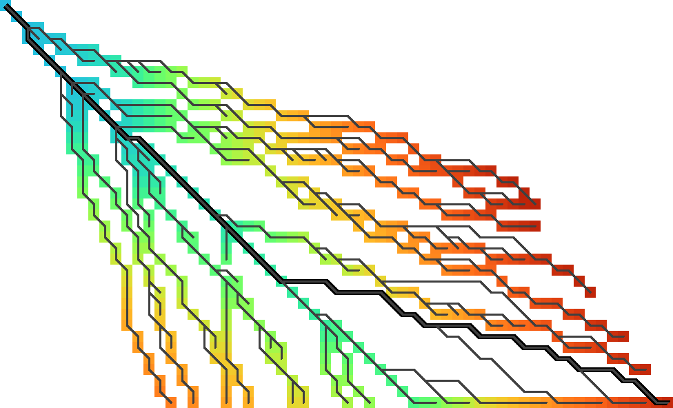
Figure 4: As in Figure 3, the coloured cells show the f.r. states computed and stored by diagonal transition. This time, the tree shows the backward greedy path traced back from each f.r. state. Note that paths diverge from the visited states.
Observations Link to heading
This section is just a blob of thoughts – parts are likely obscure and disorganised. Consider skipping to the next section A pragmatic solution, or proceed at your own risk.
Figure 5: Forward greedy traceback.
Figure 6: Backward greedy traceback.
I’m showing the same images again here on the right so I can make some remarks about this specific example while they are in view.
- The forward-greedy tracebacks exactly follow the visited states.
This is expected, since the diagonal-transition in itself is already
forward-greedy via the
extendstep. - The forward-greedy tracebacks are often nicely linear – they don’t branch much after leaving the main path. See for example the first (leftmost) three branches below the path, and the last (bottom) two branches above the path.
- For every position above the optimal path in both versions, an optimal traceback starting there contains only matches, substitutions, and deletions before joining the main path. (Note: deletions are horizontal edges.)
- There is only one horizontal edge below the optimal path where the traceback moves away from the main diagonal.
- The backward-greedy tracebacks never cross the forward-greedy paths, and never ’enter’ the ‘previous’ branch. They always stay within the same white unexplored region, until they branch back into an (indirect) parent of where they left the coloured branch.
- For forward-greedy traceback, we need to know exactly the parent value of \(f\).
- Starting anywhere outside the main path, the only information needed for backward-greedy tracing is whether we should make an insertion or deletion after greedily matching characters.
- No substitutions occur in the white regions. Backward-greedy edges there are either matches or indels.
- Forward-greedy and backward-greedy have exactly the same set of substitution edges.
- The $i$th branch on each side tells us how far we can get with \(i\) substitutions.
- More generally, substitution edges outside the main path are rare. Most diagonal edges there are matches, but those (and only those?) starting in a state where the tree splits (into multiple branches) are substitutions.
This leads me to:
- Hypothesis 1
- The tree splits at the start (top-left) of every forward-greedy substitution edge,
and every split is followed by a critical substitution edge.
A split is where a branch splits into two branches.
An edge is critical when it is included in every optimal path to the state at the end of the edge.
What information is needed for path tracing Link to heading
Let’s take another look at Figure 3 and determine the minimal information needed with which we could reconstruct tracebacks from each visited (coloured) state. (Yep, I’m just going to keep repeating this every time it scrolls out of my view ;)) The previous observations hinted at substitutions being important, so I’m highlighting those red in Table 1. (The lazy way to do side-by-side figures.) To reduce distractions, I’m removing the gradient and drawing f.r. states as grey. States that are visited while extending are lighter grey.
 |  |
The starting point will be the following. (I’m skipping a few earlier iterations with tricky issues, so this may turn out to actually work.)
- Hypothesis 2
- All tracebacks can be reconstructed from the induced sub-graph on substitution edges and branch-tips.
To expand on this: the set of all tracebacks together forms a tree, which is just a special kind of graph. Now take all states that are either at the start or end of a substitution edge, or at the tip of a branch, i.e. a leaf of the tree. The induced subgraph is the graph on these states that connects two states when they are joined by a path in the tree that does not go through any other selected states.
Let’s see how we could use this information to generate a backward greedy traceback starting at a given tip:
- Algorithm 1
- From the tip, we know the parent state that is at start/end of a substitution. The path to the parent can contain no other substitutions, and so consists of matches and indels only. Alternate backward-greedy matching with single indel steps in the right direction (i.e. towards the diagonal of the parent) until the parent is reached. Then repeat. Take a substitution step only when the state is already in the same diagonal as the parent.
This looks great! In fact, I think this can recover the entire figure above! However, there is one subtle point: it depends on the following hypothesis:
- Hypothesis 3
- The path from a visited state to its parent (that is, the first state on the traceback at either the start or end of a substitution edge) does not contains insertion edges or does not contain deletion edges. Which of the two naturally depends on whether the parent is on a diagonal above or below the current position.
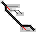
Figure 7: The optimal path contains an insertion (vertical edge) followed by matches and then a deletion (horizontal edge) without in-between substitutions.
So, let’s do some reasoning on this. Suppose the path to the parent contains both insertions and deletions. Then there is an insertion that is followed by a deletion, with at least one match in between. (An insertion directly following a deletion is never optimal.)
Figure 7 on the right shows such a case, where there is not a single substitution on the final path. Note however that the path includes two states at the start of a substitution edge: those at the start of the insertion and deletion respectively. Thus, Hypothesis 3 above reduces to this:
- Hypothesis 4
- Every time a traceback has an insertion, then matches, and then a deletion, the start of the deletion is also the start of a critical substitution edge (i.e. coloured red in our figures).
This would prevent the existence of both insertions and deletions between consecutive substitution states.
Here is where things get unsure though, because my feeling is that this can not be guaranteed. There could be … <deleted ramblings>.
.
.
Later that day: After going through many random alignments, indeed here is a counter example:
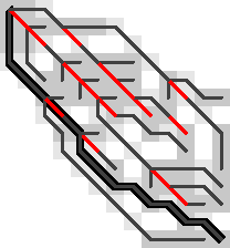
Figure 8: A counter example to Hypotheses 1, 2, 3, and 4. The optimal path contains an insertion (vertical edge) followed by two matches and then a deletion (horizontal edge). There is no critical (red) substitution edge starting at the start of the deletion, contradicting the hypotheses.
This means that starting in the bottom right, it is not sufficient to store the first substitution on the traceback as the parent: the path goes down one diagonal beyond the substitution, and then comes back up. Algorithm 1 can’t handle this, as it only walks greedily towards the parent diagonal, and never away from it.
A pragmatic solution Link to heading
To better show what is going on, I’m switching to a more complicated input: given a pattern of length \(10\), \(A\) and \(B\) are respectively \(11\) and \(6\) copies of the pattern after applying \(20\%\) of mutations. This creates repetitive strings with many good alignment candidates, Figure 9.

Figure 9: WFA on two sequences made of (11) and (6) copies of a repeating pattern with (20%) mutations applied to each. F.r. states are grey, and extended states are lighter grey. Substitutions on the tracebacks are red. Click the image to open a larger version in a new tab.
As before the idea is to remove as much information as possible while still being able to recover all tracebacks.
The first step is to throw away all matching edges. WFA also doesn’t store extended states (the light grey ones), and we easily recover them via backwards greedy matching.
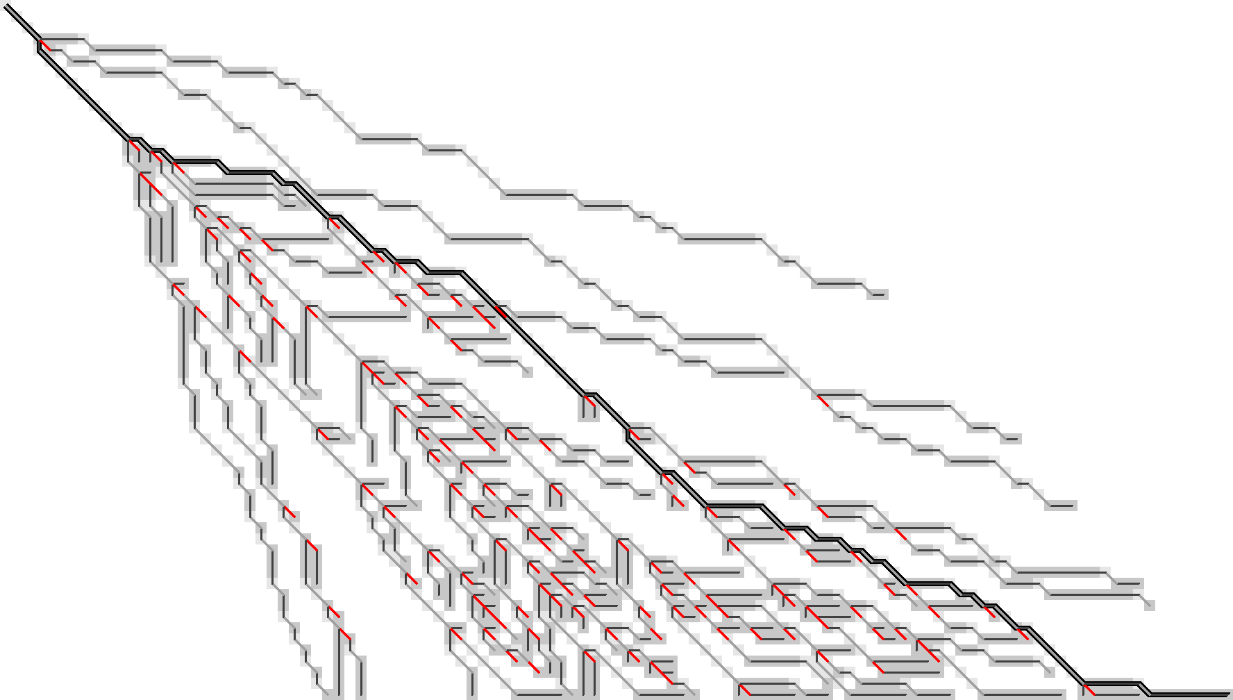
Figure 10: After discarding matching edges (made grey here) and only storing indels (black) and substitutions (red) we can still trace back all paths.
Additionally, let’s try to only preserve the substitution edges, and throw out all indel edges, Figure 11.
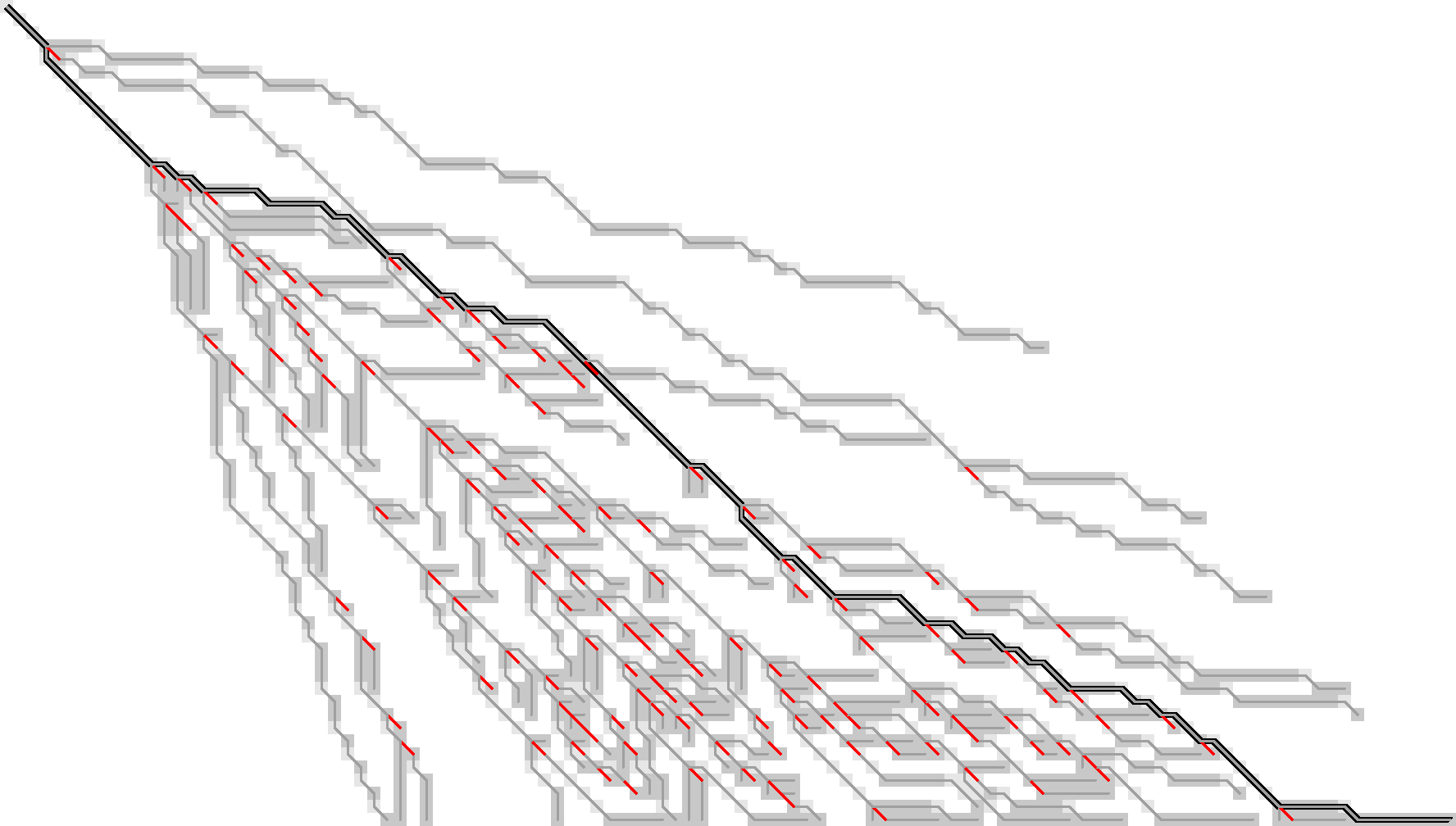
Figure 11: Here, we only store the red substitution edges.
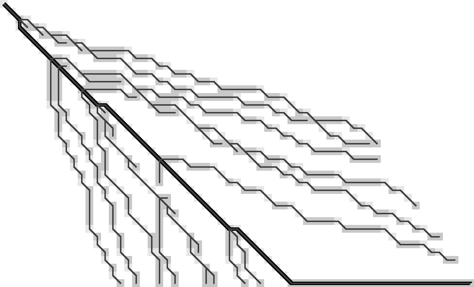
As you can see, there are still a lot of substitution edges to be stored in Figure 11. We don’t actually need all of them! Only the paths leading to an active f.r. point on the last wavefront can become part of the final shortest path. So, let’s only store the tracebacks starting from the last front, Figure 12.
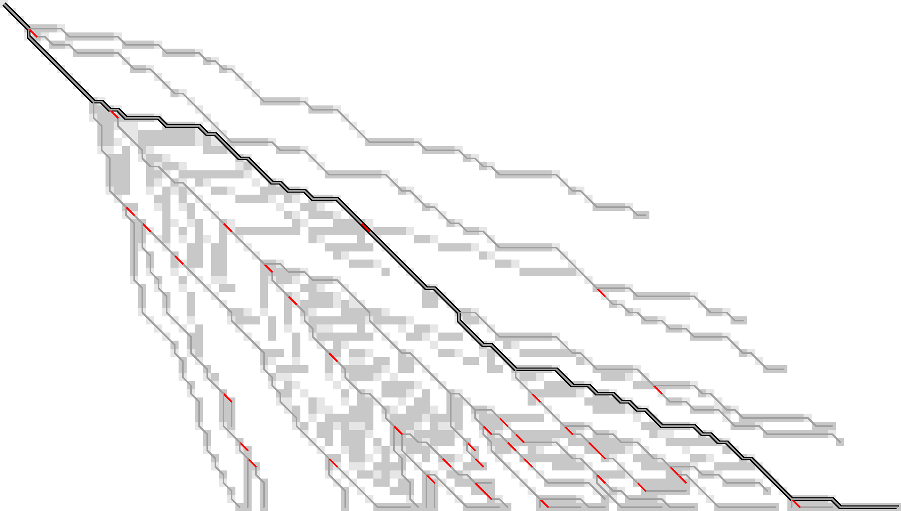
Figure 12: Storing only tracebacks from the last wavefront, there are much fewer substitutions to keep track of.
Now, we could trace the path as follows:
- Algorithm 2 (broken attempt)
- Let the parent \(f_{s’,k’}\) of a given state \(f_{s,k}\) be the f.r. point at
the start of the last (furthest) substitution on its traceback, where it is possible that
\(s’ < s-1\) and \(|k-k’| > 1\).
The path from \(f_{s,k}\) to \(f_{s’, k’}\) can be found by alternating the following steps:
Greedily match edges backwards.
Make an insertion (increasing \(k\)) if \(k’ > k\) or a deletion (decreasing \(k\)) if \(k’ < k\).
If \(k’ = k\) and we have not yet reached \(f \leq f_{s’, k’}\), make a single substitution, and then assert that we are in \(f_{s,k}\).
It turns out this algorithm is broken for the main path in Figure 12!1 Just below the middle it changes diagonals back-and-forth a few times, without a substitution to guide us. This would cause the assertion at the end of the algorithm above to fail. Thus, we need to track more information: we add in extra parent states every time a path changes diagonals back-and-forth. To be precise: Each time a path has insertions, followed by matches, followed by a deletion (or the reverse), the state at the start of the deletion is also stored as a parent state. These are blue in Figure 13.
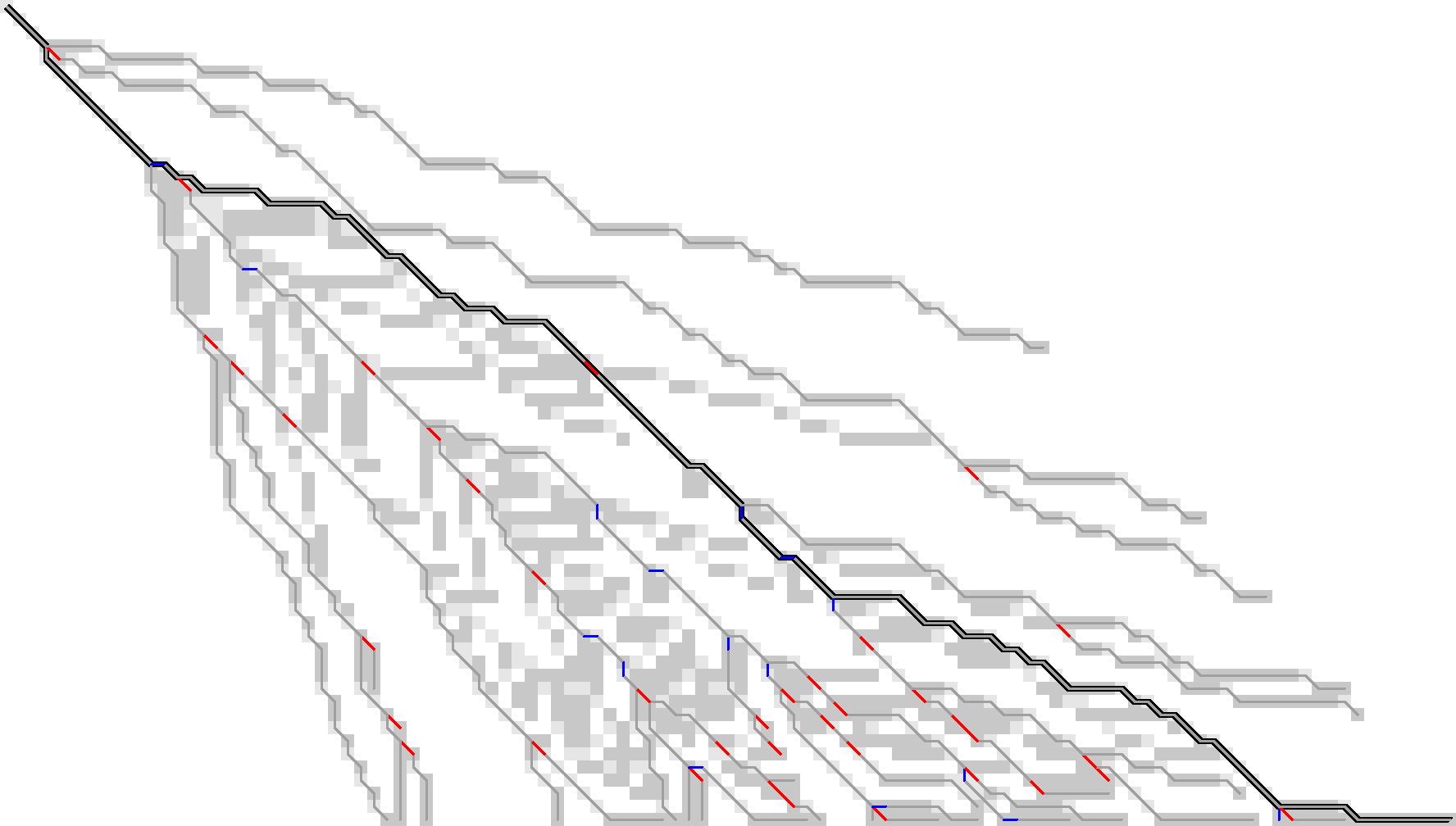
Figure 13: We additionally store indel edges when the path changes the direction of the change of diagonals. These additional edges are shown in blue. In total, for this sample we need to store around 50 parent states to have enough information to reconstruct all tracebacks.
- Algorithm 2 (fixed)
- Same as the broken attempt for Algorithm 2, but now let the parent be the start of the last red /or blue edge on the traceback.
To wrap up, here is the same data for the simpler figure we started with. In this case, only very few states (less than \(s\), in fact) need to be tracked to be able to reconstruct the traceback for all states on the last wavefront.
Figure 14: The storage needed (12 states) to generate all tracebacks in Figure 3.
Another interpretation Link to heading
Here is another way of looking at what we did so far.
Each path can be written down as a sequence of operations M (match), X
(mismatch), I (insert), and D (delete), like MXMIMIMMDDMM.
Let’s drop all the matches M, giving XIIDD. Now, let’s insert the diagonal
before each character: (0)X (0)I (-1)I (-2)D (-1)D. Now drop all I’s and
D’s, apart from those preceded by a D or I (the opposite one) respectively: (0)X (-2)D.
Let’s call this the compressed path.
The red edges from before now correspond to the X’s, and the blue edges
correspond to the D’s. Just this string is sufficient to reconstruct the
entire path: From the back, walk to the next listed diagonal while greedily
matching edges, and whenever you encounter an X, make a substitution.
Affine costs Link to heading
Note that everything so far works for both unit costs and linear costs. For affine costs, something more is needed.
In particular, the backward-greedy path tracing idea does not work in this case, since alternating insertions and deletions is not free anymore, and it is not clear when to end each affine indel.
It seems that the best we can do is to explicitly mark each affine
gap-open location, and ignore substitutions.
In terms of the CIGAR-strings above, we keep the first I and D of each run
of insertion/deletion characters, annotated with the exact location the gap opens.
Figure 15 shows the resulting stored states.
Figure 15: For affine costs, we can instead store all gap-open locations, marked in blue, and ignore the substitutions. There are roughly 65 of them.
The simpler input that we started with looks like Figure 16.
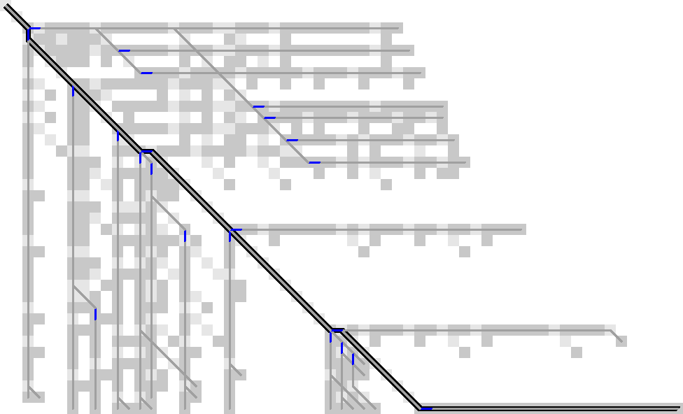
Figure 16: Gap-open locations for the test case from the start.
For completeness, the algorithm to find the traceback is as follows:
- Algorithm 3 (affine traceback)
- Given a state \(f_{s,k}\) and the last gap-open state on its path \(f_{s’, k’}\),
the path in between can be found as follows:
- Walk diagonally with matches and mismatch until reaching the row or column of the parent.
- Make an indel to the start of the gap.
Conclusion Link to heading
We have found a method to significantly reduce the amount of memory needed to store tracebacks for WFA. For simple inputs, this will likely be linear in the edit distance, \(O(s)\). For repetitive sequences with multiple good candidates, more memory may be needed, but it should still be less than the typical memory required by WFA.
Implementation. The next step here is to implement this and see how well it works in practice. While it’s relatively simple to compute the important states at the end of the algorithm (for the visualizations), doing this on the fly seems more tricky. I’m a bit worried that constantly updating the induced graph (adding new parent states; discarding parts that do not reach the last front anymore) may take longer than just the computation of each next wavefront.
Experiments. Using an implementation, we can run this on much larger inputs and see the effect it has on memory consumption. It should be evaluated on hard-to-align sequence pairs to evaluate the memory savings in such cases as well. A slightly simpler thing to do would be to only count the number of parents that needs to be stored in both the linear and affine cases.
References Link to heading
It actually took a lot of tries to find such an example. ↩︎