- Notation
- Needleman-Wunsch: where it all begins
- Dijkstra/BFS: visiting fewer states
- Band doubling: Dijkstra, but more efficient
- GapCost: A first heuristic
- Computational volumes: an even smaller search
- Cheating: an oracle gave us \(g^*\)
- A*: Better heuristics
- Broken idea: A* and computational volumes
- Local doubling
- Diagonal Transition
- A* with Diagonal Transition and pruning: doing less work
- Goal: Diagonal Transition + pruning + local doubling
- Pruning: Improving A* heuristics on the go
- Cheating more: an oracle gave us the optimal path
- TODO: aspriation windows
\begin{equation*} \newcommand{\st}[2]{\langle #1,#2\rangle} \newcommand{\g}{g^*} \newcommand{\fm}{f_{max}} \newcommand{\gap}{\operatorname{Gap}} \end{equation*}
This post is an overview/review of existing alignment algorithms, explained using visualizations. This builds up to the introduction of local doubling, an idea I had while writing a previous post on pre-pruning. My hope is that this can combine the efficiency of Needleman-Wunsch or Diagonal Transition implementations (e.g. Edlib and WFA using bitpacking and SIMD), while having the better complexity of A*-based alignment.
See also my review post on pairwise alignment, comparing algorithms and their runtime/memory trade-offs. This post aims to be visual and intuitive, while that one (as for now) is more formal/technical.
Notation Link to heading
- Input: sequences of length \(n\) and \(m\). For complexity analysis, we assume that \(m=n\).
- States of the alignment graph:
- states \(u = \st ij\),
- start \(s = \st 00\),
- end \(t = \st nm\).
- Distances:
- distance between vertices \(d(u, v)\),
- distance from start \(g = g(u) := d(s, u)\),
- gapcost: \(\gap(u, v) = \gap(\st ij, \st {i’}{j’}) = |(i’-i) - (j’-j)|\).
Needleman-Wunsch: where it all begins Link to heading
- Invented by (Needleman and Wunsch 1970) and others. See the review post.
- Visits all states \(\st ij\) of the DP table ordered by column \(i\).
- In fact, any topological sort (total order) of the states of the underlying dependency graph (partially ordered set) is allowed. One particular optimization is process anti-diagonals in order. Those correspond to anti-chains in the poset, and hence can be computed independently of each other.
- Complexity: \(O(n^2)\).
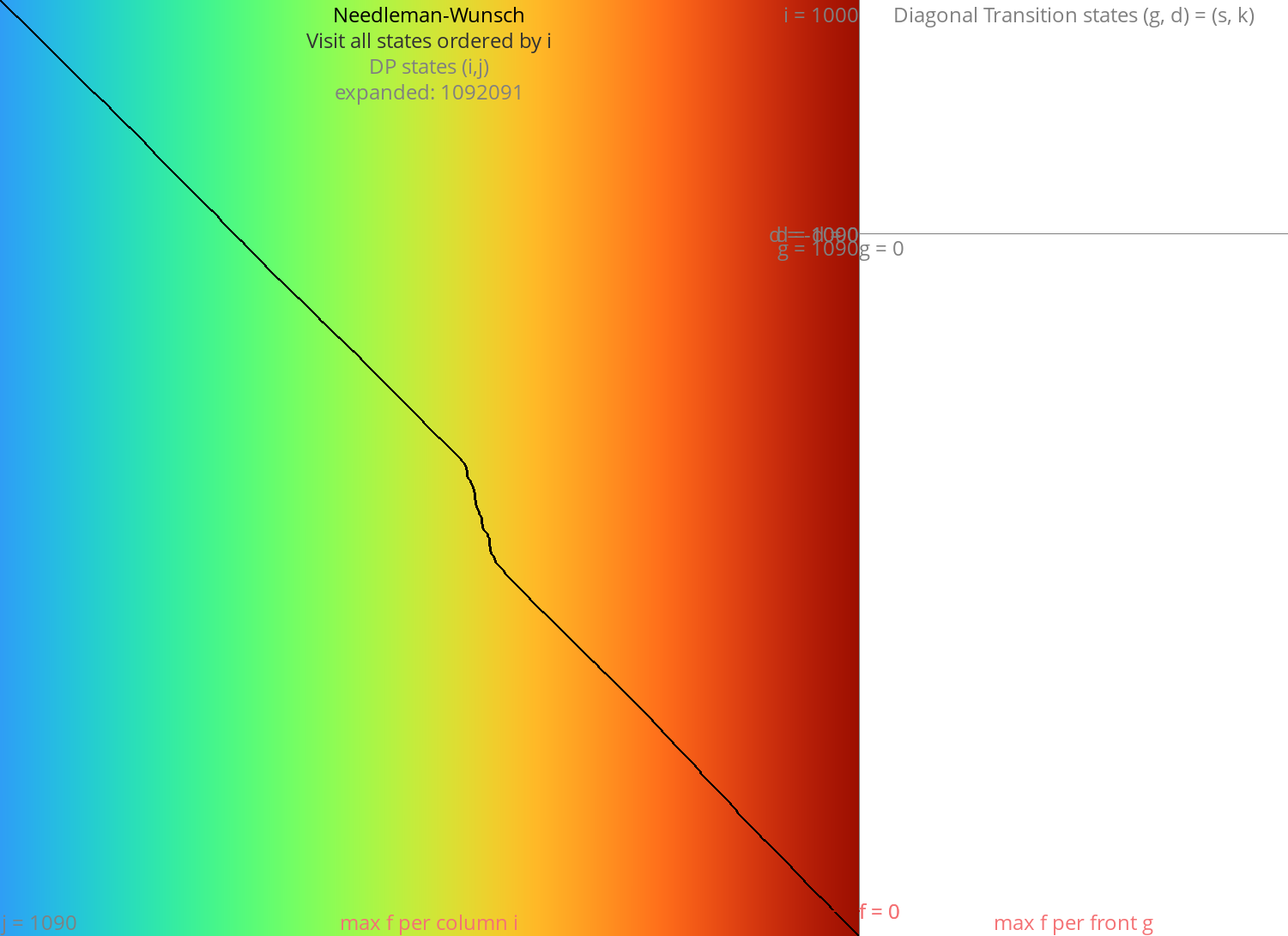
Figure 1: NW expands all 1000x1000 states. Ignore the right half for now.
Dijkstra/BFS: visiting fewer states Link to heading
Mentioned in Ukkonen (1985)
Visit states ordered by the distance from start \(s\): \(g(u) := d(s, u)\).
Visits exactly those states with
\begin{equation} g(u) \leq \g,\label{dijsktra} \end{equation}
where \(\g := d(s, t)\) is the total alignment distance.
Drawback: much slower:
- bithacks/SIMD don’t work,
- queues are slow compared to iteration.
Complexity: \(O(n d)\), where \(d=\g\) is the edit distance.
- Typical notation is \(O(ns)\) for arbitrary scores and \(O(nd)\) for edit distance. I’d use \(O(n\g)\) for consistency but it’s ugly and non-standard.
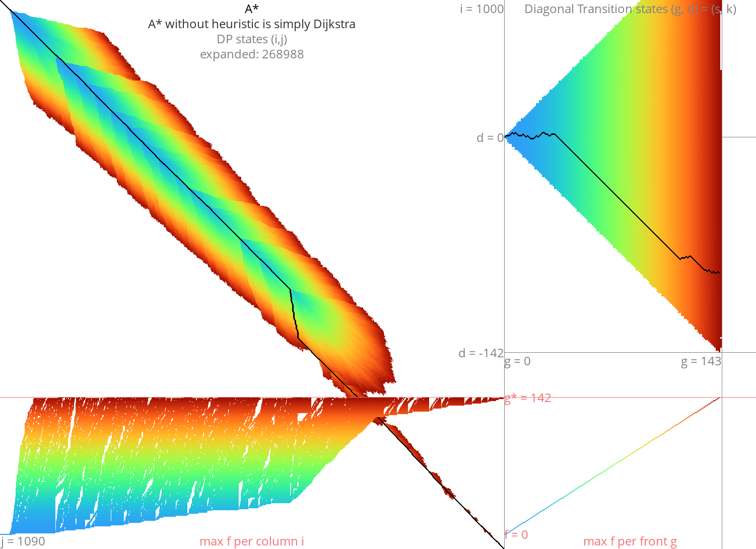
Figure 2: Dijkstra
Band doubling: Dijkstra, but more efficient Link to heading
- Introduced in Ukkonen (1985)
- Idea: use NW’s efficient column-order to compute only the states with \(g(u) \leq \g\).
- We don’t know \(\g\), but we can find it using exponential search or band doubling.
- For a guess \(\fm\) of \(\g\):
Compute all states with
\begin{equation} \gap(s, u) \leq \fm,\label{doubling} \end{equation}
where \(\gap(s, \st ij)\) is the cost of indels (gapcost) needed to go from \(s\) to \(\st ij\). For edit distance this is simply \(|i-j|\).
When \(g(t) \leq \fm\), all states with \(g\leq \g =g(t) \leq \fm\) have been computed, and we found an optimal path.
Otherwise, double the value of \(\fm\) and try again.
- Starting with \(\fm = 1\), this takes \(T:=1n + 2n + \dots + f_{last}\cdot n\) time. Since \(f_{last}/2 < \g\) we have \(T= (2f_{last}-1)n \leq 4\g n\).
- Complexity: \(O(nd)\)
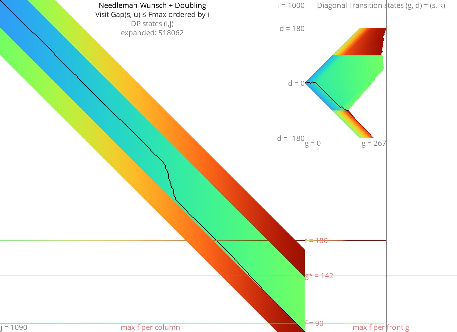
Figure 3: NW + doubling
GapCost: A first heuristic Link to heading
We can sharpen \eqref{doubling} by also bounding the indel cost (gapcost) from \(u\) to the end:
\begin{equation} \gap(s, u)+\gap(u, t) \leq \fm,\label{doubling-gap} \end{equation}
Assuming both input sequences are the same length (\(m=n\)), this halves the runtime.
This can also be used on top of Dijkstra to give a first A* variant where states are ordered by \(f(u) := g(u) + \gap(u, t)\).
It is possible to transform the insertion and deletion costs in a way that already accounts for the gapcost, see this post.
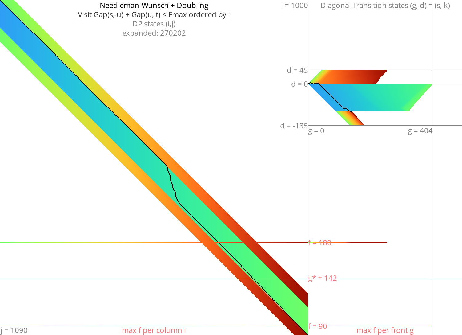
Figure 4: NW + doubling + gapcost
Computational volumes: an even smaller search Link to heading
Introduced in Spouge (1989)
Equations \eqref{doubling} and \eqref{doubling-gap} determine the area to be computed up-front. But we can make a simple improvement and take into account the current distance \(g(u) \geq \gap(s, u)\):
\begin{equation} g(u)+\gap(u, t) \leq \fm.\label{volume-gap} \end{equation}
An even simpler option is \(g(u) \leq \fm\), which corresponds directly to computing increasing portions of Dijkstra.
This still relies on repeated doubling of \(\fm\).
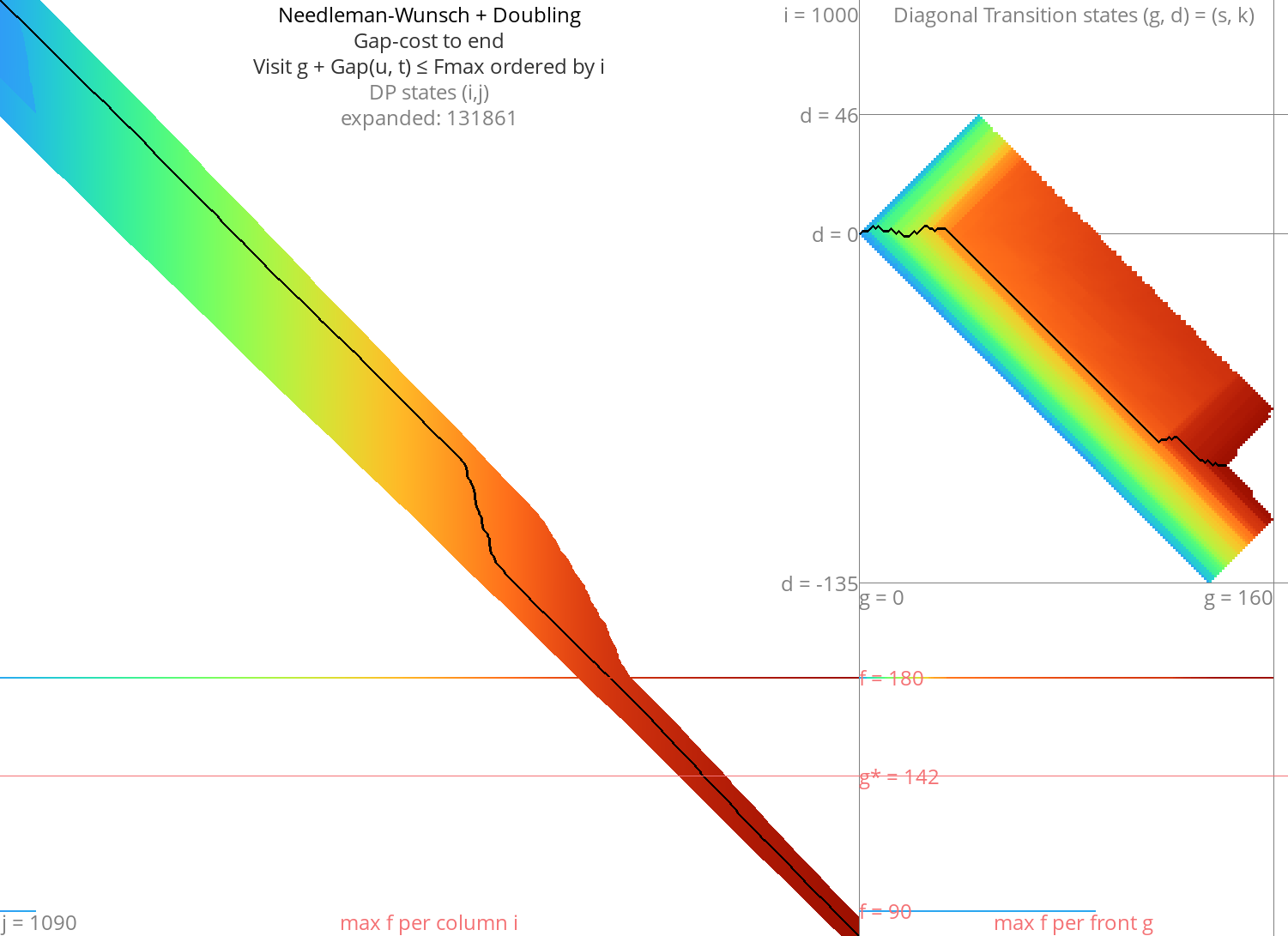
Figure 5: NW + doubling + g + gapcost
Cheating: an oracle gave us \(g^*\) Link to heading
- If we already know the target distance \(\g\), we can skip the exponential
search over \(\fm\) and directly use \(\fm = \g\). This will speed up all of the
band doubling algorithms above up to \(4\) times:
- no need to try smaller \(\fm<\g\) => \(2x\) faster,
- no more unlucky cases where \(\fm=2\g-\epsilon\).
- More generally, we can make an initial guess for \(\fm\) if we roughly know the distance distribution of the input.
A*: Better heuristics Link to heading
Instead of visiting states by column \(i\) or distance \(g\), we can order by
\begin{equation} f(u) := g(u)+h(u) \leq \g,\label{astar} \end{equation}
where \(h\) is any heuristic function satisfying \(h(u) \leq d(u, t)\).
Drawback: Again, A* is slow because of the priority queue and many computations of \(h\).
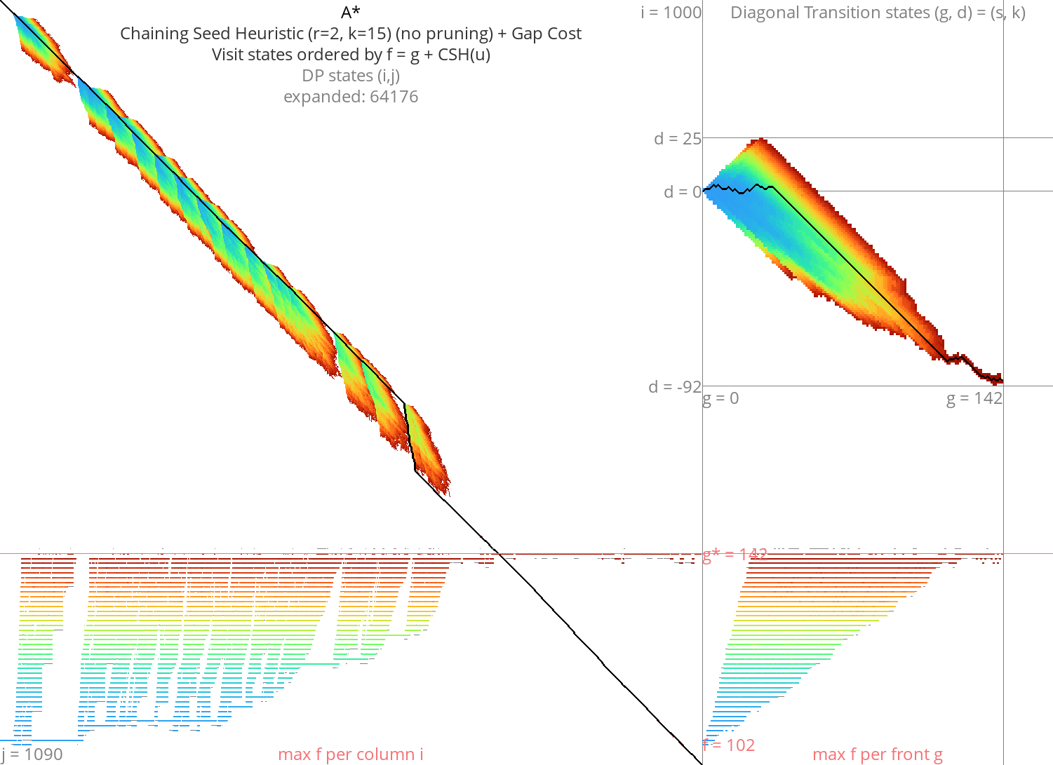
Figure 6: A* + CSH + gapcost
Broken idea: A* and computational volumes Link to heading
- Just like band doubling speeds up Dijkstra, can we use it to speed up A*?
- Start with \(\fm = h(s)\).
- Compute all states with \(f(u) \leq \fm\) in column-order.
- Double \(\fm\) after each try.
- BROKEN: If we start with \(\fm = h(s) = \g-1\) and we double to \(\fm = 2\g-2\) the number of expanded states goes from \(O(n)\) to \(O(n^2)\).
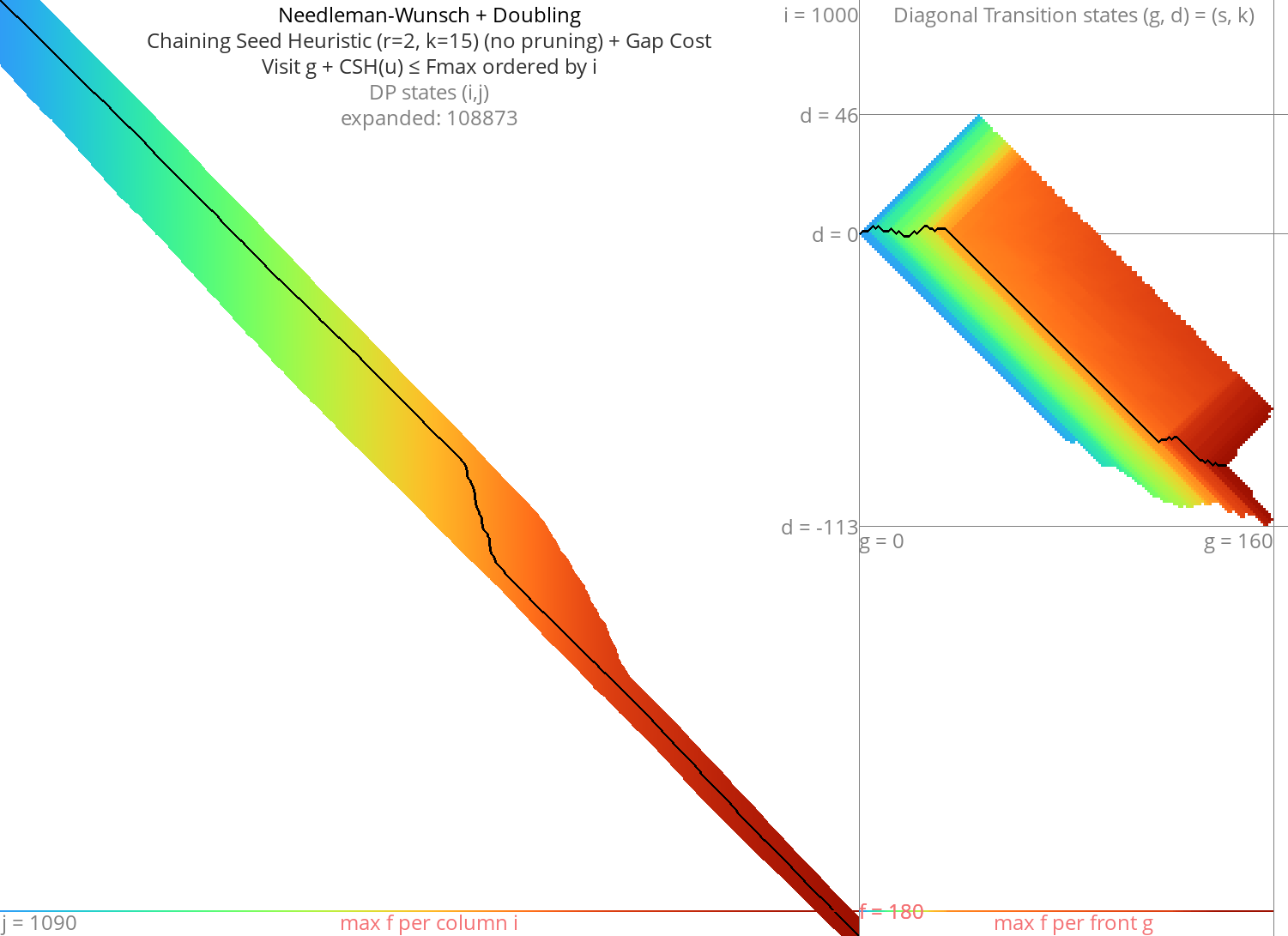
Figure 7: NW + CSH + gapcost + Doubling
Local doubling Link to heading
Without heuristic Link to heading
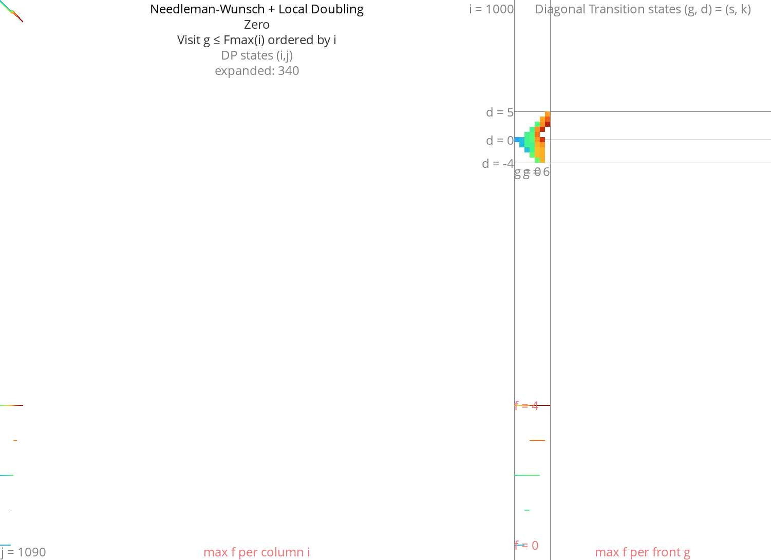
Figure 8: NW + Local-Doubling
With heuristic Link to heading
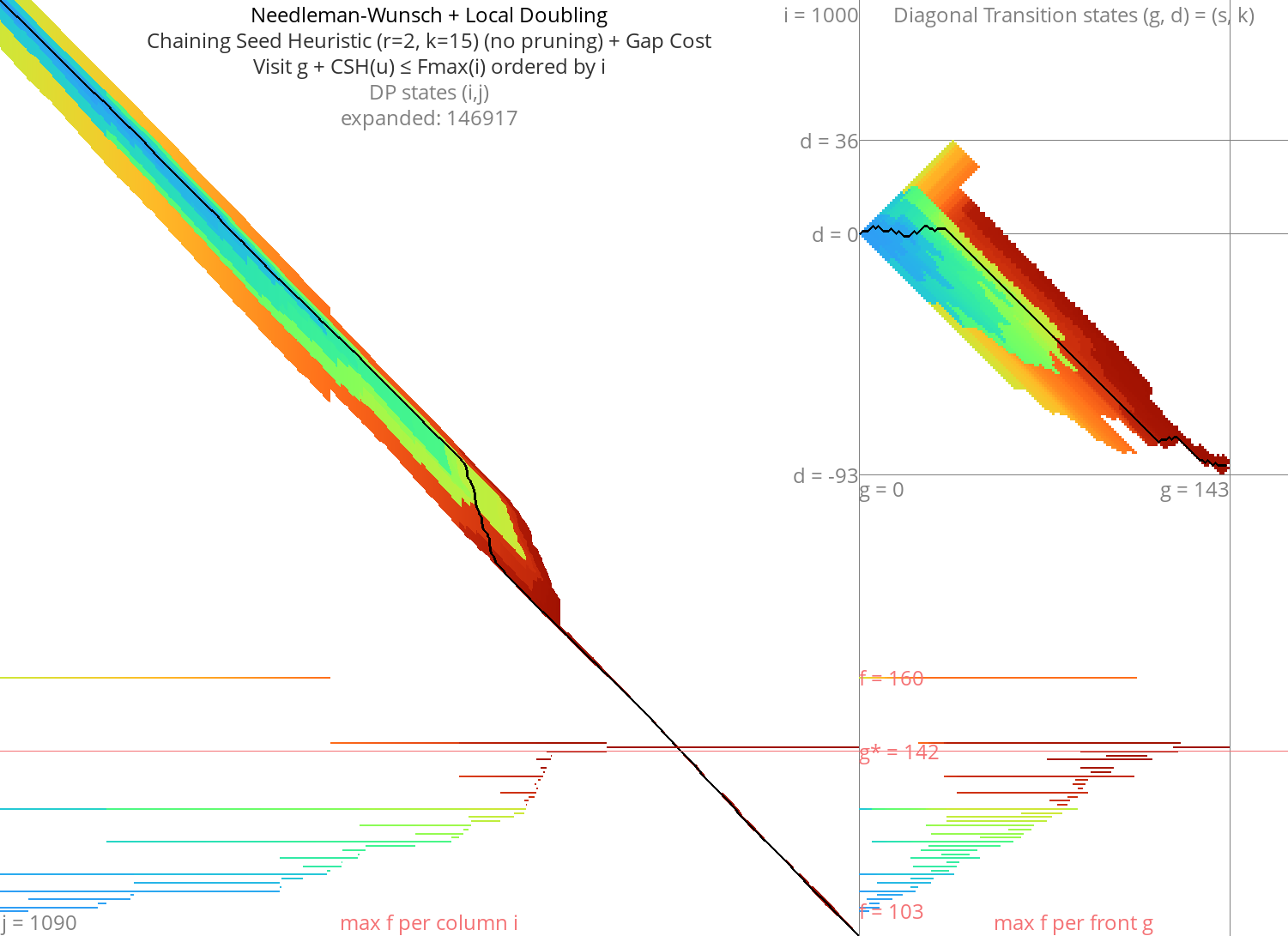
Figure 9: NW + CSH + gapcost + Local-Doubling
Diagonal Transition Link to heading
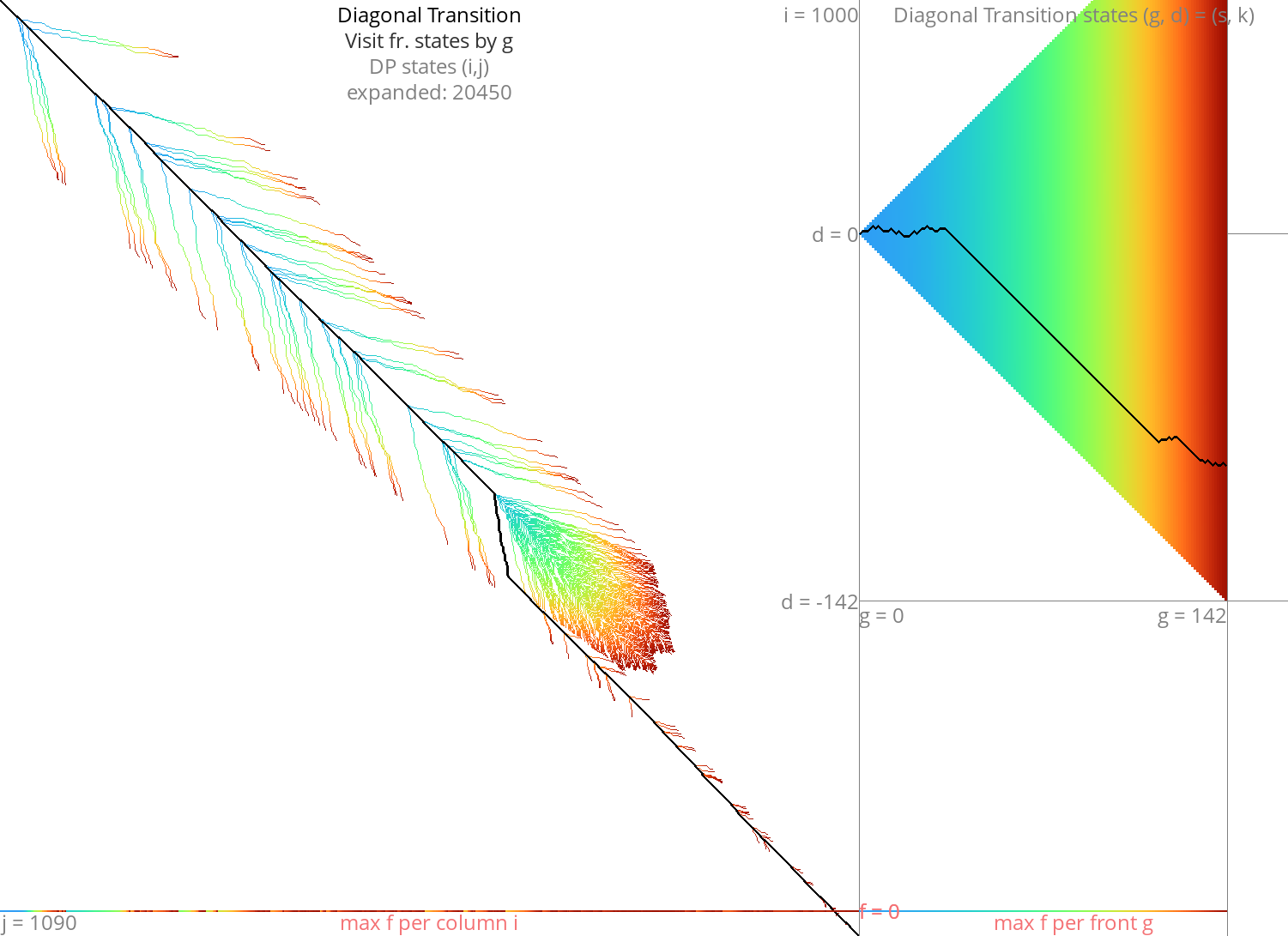
Figure 10: DT
A* with Diagonal Transition and pruning: doing less work Link to heading
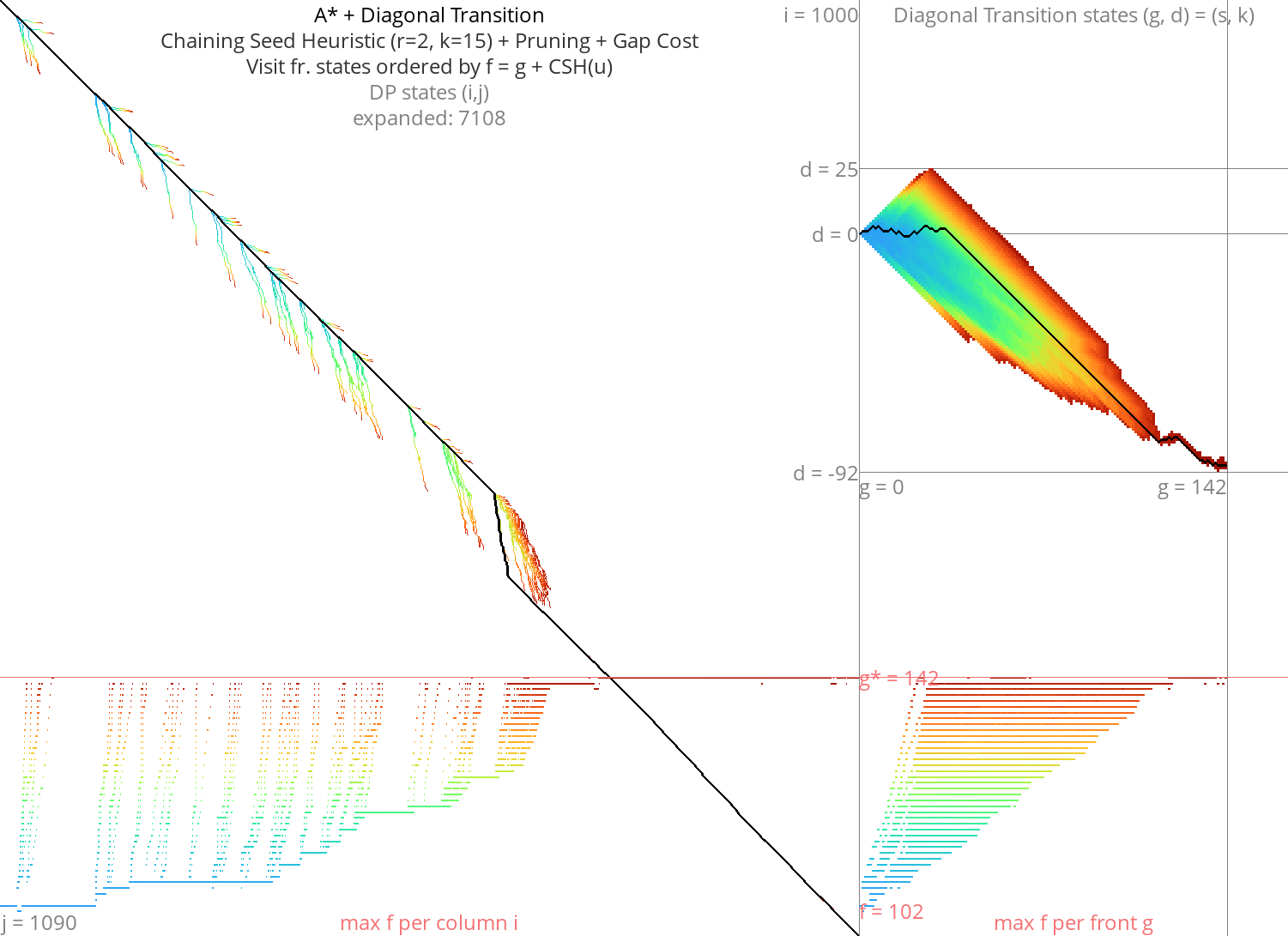
Figure 11: Astar + DT
Goal: Diagonal Transition + pruning + local doubling Link to heading
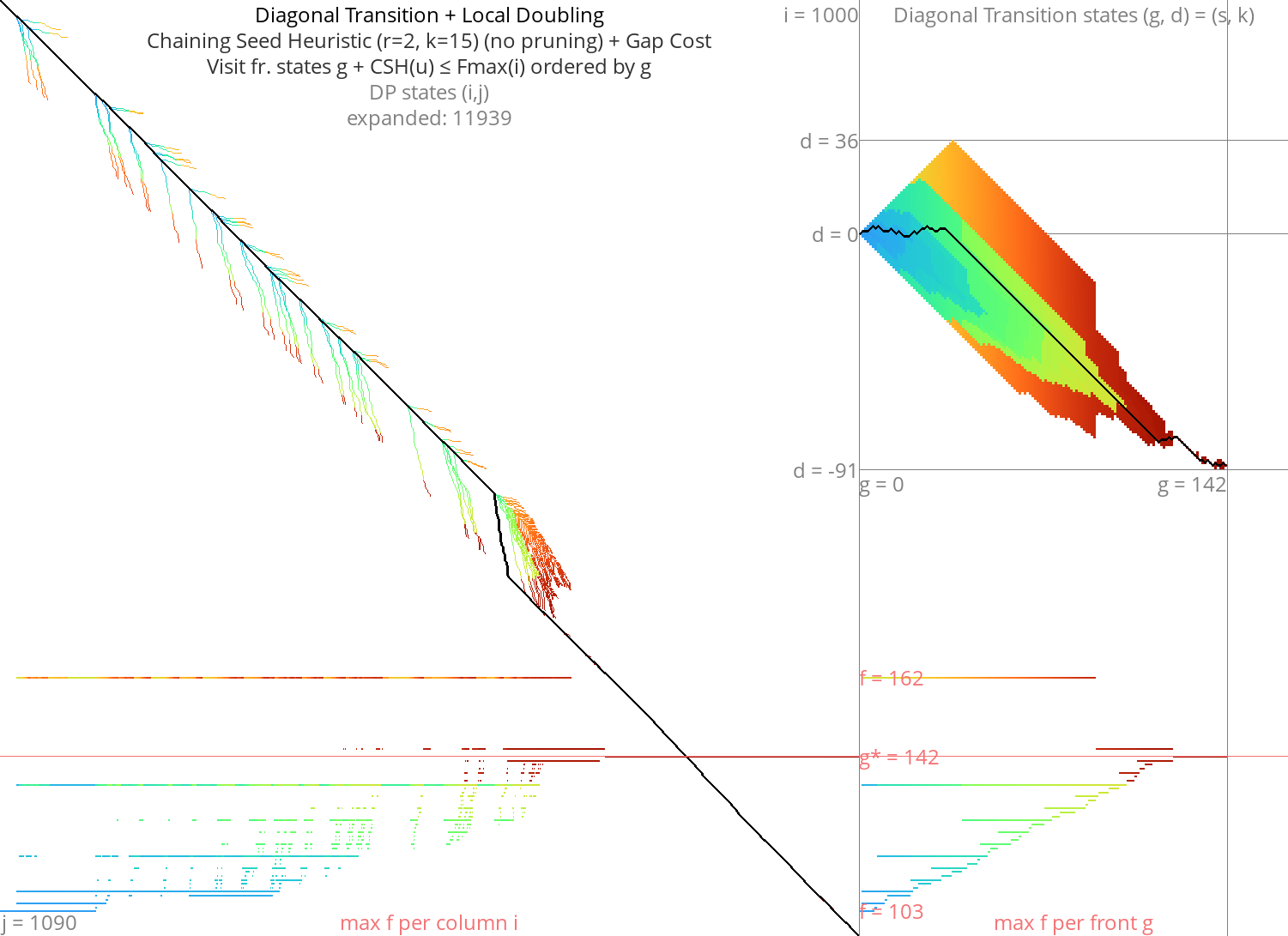
Figure 12: DT + CSH + gapcost + Local-Doubling
Here’s a gif with pruning as well:
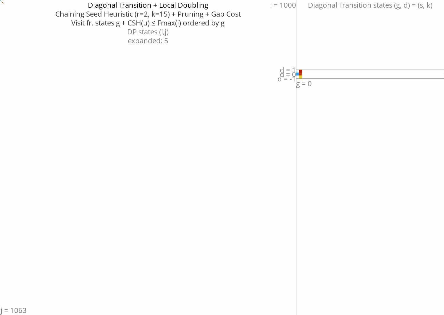
Figure 13: DT + CSH + gapcost + pruning + Local-Doubling
Pruning: Improving A* heuristics on the go Link to heading
Cheating more: an oracle gave us the optimal path Link to heading
- Pruning brings a challenge to the local
TODO: aspriation windows Link to heading
In chess engines (ie alpha beta search/pruning) there is the concept of aspiration window which is similar to exponential search. Maybe we can reuse some concepts.