This is Part 2 of my thesis (Groot Koerkamp 2025), containing chapters 6 to 9 on Low Density Minimizers. Please cite the thesis instead of this post.
1 Theory of Sampling Schemes Link to heading
In this chapter, we introduce minimizers, and more general sampling schemes. These are methods to sample a subset of \(k\)-mers from a text in a deterministic way, such that at least one \(k\)-mer is sampled from every string of length \(k+w-1\), for some window guarantee \(w\).
A key property of such schemes is their density: how few \(k\)-mers can be sampled while still respecting the window guarantee. Applications benefit from a lower density, since this usually means indices on the text are smaller.
We cover a number of theoretical results from the literature, and explain how the density of a minimizer scheme can be computed. This will serve as the background for the following two chapters, that go deeper into lower bounds on sampling scheme density and practical sampling schemes.
In this chapter, we survey existing literature on minimizers. Small parts of this chapter are loosely based on the background sections of the mod-minimizer papers (Groot Koerkamp and Pibiri 2024; Groot Koerkamp, Liu, and Pibiri 2025), written with Giulio Ermanno Pibiri and Daniel Liu, and the density lower bound paper (Kille et al. 2024), written with Bryce Kille and others. Specifically some definitions and theorem statements are copied verbatim.
\[ \newcommand{\O}{\mathcal O} \newcommand{\order}{\mathcal O} \newcommand{\Ok}{\mathcal O_k} \newcommand{\Ot}{\mathcal O_t} \newcommand{\Os}{\mathcal O_s} \newcommand{\Dk}{\mathcal D_k} \newcommand{\Dtk}{\tilde{\mathcal D}_k} \newcommand{\P}{\mathbb P} \newcommand{\pr}{\mathbb P} \DeclareMathOperator*{\argmin}{argmin} \DeclareMathOperator*{\poly}{poly} \DeclareMathOperator*{\revcomp}{rc} \DeclareMathOperator*{\sparsity}{sparsity} \newcommand{\ceil}[1]{\left\lceil{#1}\right\rceil} \newcommand{\floor}[1]{\left\lfloor{#1}\right\rfloor} \newcommand{\c}{\mathrm{c}} \newcommand{\boldremuval}{\mathbf{ReM}_{\mathbf{u}}\mathbf{val}} \newcommand{\remuval}{\mathrm{ReM}_{\mathrm{u}}\mathrm{val}} \]
1.1 Introduction Link to heading
As does nearly every paper in bioinformatics, we will start here with the remark that the amount of biological data has been and still is increasing rapidly over time. Thus, both faster and more space efficient algorithms are needed to analyse this data. One popular method for sequence analysis is to consider a sequence as its set of \(k\)-mers, i.e., the set of substrings of length \(k\), which often has a value up to \(31\). Then, two sequences can be compared by comparing these sets, rather than by doing a costly alignment between them. For example, when comparing two human genomes, there will likely be relocations and inversions of long segments of DNA, so that a global alignment is not the best way forward. By instead only considering \(k\)-mers, we only consider the local structure, so that the changes in global structure do not affect the analysis. Then one could estimate the similarity of these sets using min-hash (Broder 1997; Kille et al. 2023). Or one could seed an alignment by finding \(k\)-mer matches between the two sequences, as done by minimap (Li 2016).
A drawback of considering the full set of \(k\)-mers is that consecutive
\(k\)-mers overlap, and thus that there is a lot of redundancy.
To compress the set of \(k\)-mers,
it would be preferable to only sample every \(k\)’th \(k\)-mer, so that each
base is covered only exactly once. That, however, doesn’t work:
if we are given two sequences, but one is shifted by one due to an inserted base
at the very start, no common \(k\)-mers will be sampled.
To fix this, we would like a locally consistent sampling method, that decides
whether or not to sample a \(k\)-mer only based on the \(k\)-mer and some
surrounding context. One option is to use all \(k\)-mers that start with an A,
or to use all \(k\)-mers whose (lexicographic or hashed) value is sufficiently small.
Indeed, this approach is sufficient for some applications.
A drawback of the methods so far is that there could be long stretches of input without any sampled \(k\)-mers. This can cause long gaps when seeding alignments. Also when building text indices, such as a sparse suffix array (Grabowski and Raniszewski 2017; Ayad, Loukides, and Pissis 2023) or a minimizer-space De Bruijn graph (Ekim, Berger, and Chikhi 2021), we usually need a guarantee that at least one \(k\)-mer is sampled every, say, \(w\) positions.
Sampling scheme. This brings us to local sampling schemes that satisfy a window guarantee: given a window of \(w\) \(k\)-mers, consisting of \(w+k-1\) characters, a sampling scheme returns one of the \(k\)-mers as the one to be sampled. If we now slide this window along the input, we collect the set of sampled \(k\)-mers. Ideally the scheme ensures that the same \(k\)-mer is sampled from adjacent windows, so that this set is much smaller than the total number of \(k\)-mers.
Given such a sampling scheme, we can build a locality sensitive hash: given a string of length \(w+k-1\), we can hash it to its sampled \(k\)-mer. This way, adjacent strings are likely to have the same hash, allowing for efficient indices such as LPHash and SSHash (Pibiri, Shibuya, and Limasset 2023; Pibiri 2022).
Problem statement. The goal now is to find \(k\)-mer sampling schemes that satisfy the \(w\) window guarantee, while overall sampling as few \(k\)-mers as possible.
This is formalized in the density: the expected fraction of \(k\)-mers sampled by a scheme. The window guarantee imposes a trivial lower bound of \(1/w\), since at least every \(w\)’th \(k\)-mer must be sampled.
The most common practical scheme is the random minimizer (Roberts et al. 2004; Schleimer, Wilkerson, and Aiken 2003), which hashes all \(k\)-mers in the window, and chooses the smallest one, as shown in Figure 1. This has a density of \(2/(w+1)\), roughly twice as large as the trivial lower bound.

Figure 1: An example of the random minimizer. First all (k)-mers of length (k=5) are hashed using a random hash function, as shown by the black lines with their hash written above them. Then, in each window of (w=4) consecutive (k)-mer hashes, as e.g. the window highlighted in yellow, the (position of) the smallest (k)-mer hash is recorded. Then, the (positions of) the smallest (k)-mers in all windows form the set of minimizers. This figure is taken from (Groot Koerkamp and Martayan 2025) and made in collaboration with Igor Martayan.
Now, you may ask whether it’s worth the effort to at best save a factor two of memory and speed, and you would not be alone. I asked myself this same question long before becoming interested in minimizers (at RECOMB 2022):
Why would we even care about better minimizer? We have this simple and fast random minimizer that’s only at most \(2\times\) away from optimal. Why would anyone invest time in optimizing this by maybe 25%? There are so much bigger gains possible elsewhere.
Even worse, in practice, most schemes do not (and as we will see, can not) give more than a 20% saving in density on top of the very simple random minimizer.
As we will prove in 2, when \(k\leq w+1\), we can never expect more than around 25% lower density than the random minimizer, and thus, existing schemes are already relatively close to optimal from a practical point of view. Given this new lower bound, maybe the answer is that, indeed, we should stop searching for further schemes.
Nevertheless, there is a lot of pretty maths to be found, both in the lower bounds, and in the many sampling schemes we will review and develop ourselves. Furthermore, as we will see with the mod-minimizer, when \(k>w\), we can often achieve this 25% lower density using only slightly more code, so nearly for free. Likewise, for smaller \(k\geq w\), we will see that choosing a specific order of the alphabet can improve the density of the random minimizer by over 10%, while simplifying the code. Thus, even though improvements may seem small, searching for simple sampling schemes with near-optimal density is a fruitfull research area.
1.2 Overview Link to heading
This part on minimizers is split into four chapters.
Here, in Chapter 1.3, we review the existing theory of sampling schemes. This covers, for example, local, forward, and minimizer schemes, the density of the random minimizer, and a number of theoretical results on the optimal asymptotic density of schemes as \(k\to\infty\) or \(w\to\infty\).
In Chapter 2, we go over existing lower bounds. We start at the original one of Schleimer et al. (Schleimer, Wilkerson, and Aiken 2003), that turns out to make overly strong assumptions, and end with the new nearly tight lower bound of (Kille et al. 2024).
Then, in Chapter 3, we summarize and compare existing sampling schemes, and introduce two new sampling schemes: the open-closed minimizer and the general mod-minimizer (Groot Koerkamp and Pibiri 2024; Groot Koerkamp, Liu, and Pibiri 2025). The most important result is that the mod-minimizer achieves density \(1/w\) in the limit where \(k\to\infty\), and that this convergence is close to optimal.
Lastly, in Chapter 4, we consider the special case where \(k=1\). Here, we first introduce the bd-anchor, and then improve this into the sus-anchor with anti-lexicographic sorting. This has density very close to optimal for alphabet size \(\sigma=4\), and raises the question whether perfectly optimal selection schemes can be constructed.
Many of the existing papers on sampling schemes touch more than one of these topics, as they both develop some new theory and introduce a new sampling scheme. These results are thus split over the applicable sections.
Previous reviews. This chapter is written from a relatively theoretical perspective, and focuses on the design of low-density sampling schemes. The review of Zheng et al. (Zheng, Marçais, and Kingsford 2023) takes a more practical approach and compares applications, implementations, and metrics other than just the density. It limits itself to minimizers, rather than more general local or forward schemes. A second review of Ndiaye et al. (Ndiaye et al. 2024) focuses specifically on applications, and details how minimizers are used in various tools and domains of bioinformatics.
1.3 Theory of sampling schemes Link to heading
The theory of minimizer schemes started with two independent papers proposing roughly the same idea: winnowing (Schleimer, Wilkerson, and Aiken 2003) in 2003 and minimizers (Roberts et al. 2004) in 2004. At the core, the presented ideas are very similar: to deterministically sample a \(k\)-mer out of each window of \(w\) consecutive \(k\)-mers by choosing the ‘‘smallest’’ one, according to either a random or lexicographic order. The window guarantee is a core property of minimizers: it guarantees that consecutive minimizers are never too far away from each other. Further, these schemes are local: whether a \(k\)-mer is sampled as a minimizer only depends on a small surrounding context of \(w-1\) characters, and not on any external context. This enables the use of minimizers for locality sensitive hashing (Pibiri, Shibuya, and Limasset 2023; Pibiri 2022), since the minimizer is a deterministic key (hash) that is often shared between adjacent windows.
While the winnowing paper was published first, the ‘minimizer’ terminology is the one that appears to be used most these days. Apart from terminology, also notations tend to differ between different papers. Here we fix things as follows.
1.4 Notation Link to heading
Throughout this chapter, we use the following notation.
For \(n\in \mathbb N\), we write \([n]:=\{0, \dots, n-1\}\).
The alphabet is \(\Sigma = [\sigma]\) and has size \(\sigma =2^{O(1)}\), so that each character can
be represented with a constant number of bits. For all evaluations we will
use the size-4 DNA alphabet, but for examples we usually use
the plain ABC..XYZ alphabet.
Given a string \(S\in \Sigma^*\), we write \(S[i..j)\) for the sub-string starting at
the \(i\)’th character, up to (and not including) the \(j\)’th character, where both
\(i\) and \(j\) are 0-based indices.
A \(k\)-mer is any (sub)string of length \(k\).
In the context of minimizer schemes, we have a window guarantee \(w\) indicating that at least one every \(w\) \(k\)-mers must be sampled. A window is a string containing exactly \(w\) \(k\)-mers, and hence consists of \(\ell:=w+k-1\) characters. We will later also use contexts, which are sequences containing two windows and thus of length \(w+k\).
1.5 Types of sampling schemes Link to heading
Given parameters \(w\) and \(k\), a window is a string containing exactly \(w\) \(k\)-mers, i.e., of length \(\ell = w+k-1\).
For \(w\geq 1\) and \(k\geq 0\), a local scheme is a function \(f: \Sigma^\ell \to [w]\). Given a window \(W\), it samples the \(k\)-mer \(W[f(W)..f(W)+k)\).
In practice, we usually require \(w\geq 2\) and \(k\geq 1\), as some theorems break down at either \(w=1\) or \(k=0\) (even though theoretically those parameters make sense: we can either sample every position when \(w=1\), or for \(k=0\) sample the empty substring following the final character). When \(k \geq w\), such a scheme ensures that every single character in the input is covered by at least one sampled \(k\)-mer.
A local scheme is forward when for any context \(C\) of length \(\ell+1\) containing windows \(W=C[0..\ell)\) and \(W’=C[1..\ell+1)\), it holds that \(f(W) \leq f(W’)+1\).
Forward scheme have the property that as the window \(W\) slides through an input string \(S\), the position in \(S\) of the sampled \(k\)-mer never decreases.
An order \(\Ok\) on \(k\)-mers is a function \(\Ok : \Sigma^k \to \mathbb R\), such that for \(x,y\in \Sigma^k\), \(x\leq _{\Ok} y\) if and only if \(\Ok(x) \leq \Ok(y)\).
A minimizer scheme is defined by a total order \(\Ok\) on \(k\)-mer and samples the leftmost minimal \(k\)-mer in a window \(W\), which is called the minimizer: \[ f(W) := \argmin_{i\in [w]} \Ok(W[i..i+k)). \]
Minimizer schemes are always forward, and thus we have the following hierarchy \[ \textrm{minimizer schemes} \subseteq \textrm{forward schemes} \subseteq \textrm{local schemes}. \] There are two particularly common minimizer schemes, the lexicographic minimizer (Roberts et al. 2004) and the random minimizer (Schleimer, Wilkerson, and Aiken 2003).
The lexicographic minimizer is the minimizer scheme that sorts all \(k\)-mers lexicographically.
The random minimizer is the minimizer scheme with a uniform random total order \(\Ok\).
Following (Zheng, Kingsford, and Marçais 2021a), we also define a selection scheme, as opposed to a sampling scheme. Note though that this distinction is not usually made in other literature.
A selection scheme is a sampling scheme with \(k=1\), and thus samples any position in a window of length \(w+k-1=w\). Like sampling schemes, selection schemes can be either local or forward.
We will consistently use select when \(k=1\), and sample when \(k\) is arbitrary. When \(k=1\), we also call the sampled position an anchor, following bd-anchors (Loukides, Pissis, and Sweering 2023). Note that a minimizer selection scheme is not considered, as sampling the smallest character can not have density below \(1/\sigma\).
Given a string \(S\) of length \(n\), let \(W_i := S[i..i+\ell)\) for \(i\in [n-\ell+1]\). A sampling scheme \(f\) then samples the \(k\)-mers starting at positions \(M:=\{i+f(W_i) \mid i\in [n-\ell+1]\}\). The particular density of \(f\) on \(S\) is the fraction of sampled \(k\)-mers: \(|M|/(n-k+1)\).
The density of a sampling \(f\) is defined as the expected particular density on a string \(S\) consisting of i.i.d. random characters of \(\Sigma\) in the limit where \(n\to\infty\).
Since all our schemes must sample at least one \(k\)-mer from every \(w\) consecutive positions, they naturally have a lower bound on density of \(1/w\).
As we will see, for sufficiently large \(k\) the density of the random minimizer is \(2/(w+1) + o(1/w)\). There is also the notion of density factor (Marçais et al. 2017), which is defined as \((w+1)\cdot d(f)\). Thus, random minimizers have a density factor of \(2\). While this is convenient, we refrain from using density factors here, because it would be more natural to relate the density to the lower bound of \(1/w\) instead, and use \(w\cdot d(f)\). Specifically, as defined, the density factor can never reach the natural lower bound of \(1\), because \((w+1)\cdot \frac 1w = 1+1/w > 1\).
Now that we have defined the density, the natural question to ask is:1
What is the lowest density that can be achieved by a minimizer, forward, or local scheme?
Since the classes of forward and local schemes are larger, they can possibly achieve lower densities, but by how much? The ideal is to answer some of these questions by proving a lower bound and providing a scheme that has density equal to this lower bound, ideally for all parameters, but otherwise for a subset. We can also ask what happens when \(w\to \infty\) (for \(k\) fixed), or when \(k\to\infty\) (for \(w\) fixed)? And how does this depend on the alphabet size? Or maybe we can not quite make schemes that exactly match the lower bound, but we can make schemes that are within 1% of the lower bound, or that are asymptotically a factor \(1+o(1)\) away.
There are also different parameter regimes to consider: small \(k=1\) or \(k<\log_\sigma(w)\), slightly larger \(k\leq 10\), and more practical \(k\) up to \(\approx 30\), or even larger \(k\) in theory. Similarly, we can consider small \(w\leq 10\), but also \(w\approx 1000\) is used in practice. The alphabet size will usually be \(\sigma=4\), but also this can vary and can be \(\sigma=256\) for ASCII input.
If we do find (near) optimal schemes, we would like these to be pure in some way: ideally we can provide a simple analysis of their density, as opposed to only being able to compute it without any additional understanding. This somewhat rules out solutions found by brute force approaches, as they often do not provide insight into why they work well. This motivates the following definition.
A sampling scheme is pure when it can be implemented in \(O(\poly(w+k))\) time and space.
1.6 Computing the density Link to heading
The density of a sampling scheme is defined as the expected particular density on an infinitely long string. In practice, we can approximate it closely by simply computing the particular density on a sufficiently long random string of, for example, 10 million characters.
The following theorem forms the basis for computing the density of schemes exactly (Lemma Marçais et al. 2017, 4)(Zheng, Kingsford, and Marçais 2020):
For forward schemes, a context is a string of length \(c = w+k\), consisting of two overlapping windows.
For a sampling scheme \(f\), a context \(C\) is charged when two different positions are sampled from the first and second window, i.e., \(f(C[0..w+k-1)) \neq 1+f(C[1..w+k))\).
For a local scheme, a context has length \(2w+k-1\) instead (Zheng, Kingsford, and Marçais 2021a, 3.1)(Kille et al. 2024, 3.2), and is charged when the last window samples a \(k\)-mer not sampled by any of the previous contained windows. This larger context is necessary because a local scheme can jump backwards. In practice, this
As a small variant on this a window is charged when it is the first window to sample a \(k\)-mer (Schleimer, Wilkerson, and Aiken 2003).
The density of a forward scheme equals the probability that, in a uniform random context of length \(c=w+k\), two different \(k\)-mers are sampled from the two windows, i.e., the probability that the context is charged.
Thus, the density can be computed exactly as the fraction of all \(\sigma^{w+k}\) contexts that is charged.
We can also approximate the density by sampling sufficiently many random contexts. A somewhat more efficient method is to use a De Bruijn sequence instead. A De Bruijn sequence of order \(c\) is any circular sequence of length \(\sigma^c\) that contains every sequence of length \(c\) exactly once (De Bruijn 1946). We have the following theorem, again by (Lemma Marçais et al. 2017, 4):
The density of any forward scheme equals its particular density on an order \(c=w+k\) De Bruijn sequence. For local schemes, the order \(c=2w+k-2\) De Bruijn sequence must be used instead.
Another approach, that follows from the first, is by considering cycles of length \(c\), rather than just strings of length \(c\).
The density of any forward scheme equals its average particular density over all cyclic strings of order \(c=w+k\) for forward schemes and \(c=2w+k-2\) for local schemes.
1.7 The density of random minimizers Link to heading
As a warm-up, we will compute the density of the random minimizer. We mostly follow the presentation of (Zheng, Kingsford, and Marçais 2020).
We start by analysing when a context is charged (Lemma Zheng, Kingsford, and Marçais 2020, 1).
For a minimizer scheme, a context is charged if and only if the smallest \(k\)-mer in the context is either the very first, at position \(0\), or the very last, at position \(w\).
The context contains \(w+1\) \(k\)-mers, the first \(w\) of which are in the first window, say \(W\), and the last \(w\) of which are in the second window, say \(W’\).
When the (leftmost) overall smallest \(k\)-mer is either the very first or very last \(k\)-mer, the window containing it chooses that \(k\)-mer, and the other window must necessarily sample a different \(k\)-mer. On the other hand, when the smallest \(k\)-mer is not the very first or very last, it is contained in both windows, and both windows will sample it.
Before computing the actual density, we need to bound the probability that a window contains two identical \(k\)-mers (Lemma Zheng, Kingsford, and Marçais 2020, 9).
For any \(\varepsilon > 0\), if \(k > (3+\varepsilon) \log_\sigma ( c)\), the probability that a random context of \(c\) \(k\)-mers contains two identical \(k\)-mers is \(o(1/c)\).
For any two non-overlapping \(k\)-mers in the window, the probability that they are equal is \(\sigma^{-k} \leq 1/c^{3+\varepsilon} = o(1/c^3)\). It can be seen that the same holds when two \(k\)-mers overlap by \(d>0\) characters.
There are \(c^2\) pairs of \(k\)-mers, so by the union bound, the probability that any two \(k\)-mers are equal is \(o(1/c)\).
In practice, \(k > (2+\varepsilon) \log_\sigma( c)\) seems to be sufficient, but this has not been proven yet. Even stronger, for most applications of the lemma, \(k>(1+\varepsilon)\log_\sigma( c)\) appears sufficient.
This leads us to the density of the random minimizer (Theorem Zheng, Kingsford, and Marçais 2020, 3), which is a more refined version of the simple density of \(2/(w+1)\) that was obtained in (Schleimer, Wilkerson, and Aiken 2003) and (Roberts et al. 2004).
For \(k>(3+\varepsilon)\log_\sigma(w+1)\), the density of the random minimizer is \[ \frac{2}{w+1} + o(1/w). \]
Consider a uniform random context \(C\) of \(w+k\) characters and \(w+1\) \(k\)-mers. When all these \(k\)-mers are distinct, the smallest one is the first or last with probability \(2 / (w+1)\). When the \(k\)-mers are not all distinct, this happens with probability \(o(1/w)\), so that the overall density is bounded by \(2/(w+1) + o(1/w)\).
Using a more precise analysis, it can be shown that for sufficiently large \(k\), the random minimizer has, in fact, a density slightly below \(2/(w+1)\). Marçais et al. (Marçais et al. 2017) show this using universal hitting sets. Golan and Shur (Theorem Golan and Shur 2025, 4) show that the density of the random minimizer is less than \(2\) for all sufficiently large \(k\geq w\geq w_0\), where \(w_0\) is a constant that may depend on the alphabet size \(\sigma\).
It was originally conjectured that the density of \(2/(w+1)\) is the best one can do (Schleimer, Wilkerson, and Aiken 2003), but this has been refuted by newer methods, starting with DOCKS (Orenstein et al. 2017; Marçais et al. 2017). (Although it must be remarked that the original conjecture is for a more restricted class of ‘’local’’ schemes than as defined here.)
1.8 Universal hitting sets Link to heading
Universal hitting sets are an alternative way to generate minimizer schemes. They were first introduced by (Orenstein et al. 2016, 2017).
A Universal hitting set (UHS) \(U\) is an ‘‘unavoidable’’ set of \(k\)-mers, so that every window of length \(\ell=k+w-1\) contains at least one \(k\)-mer from the set.
Universal hitting sets are an example of a context-free scheme (Edgar 2021), where each \(k\)-mer is sampled only if it is part of the UHS:
A context-free scheme decides for each \(k\)-mer independently (without surrounding context) whether to sample it or not.
There is a tight correspondence between universal hitting sets and minimizer schemes (Marçais et al. 2017, 3.3)(Marçais, DeBlasio, and Kingsford 2018, 2.1.5)(Zheng, Kingsford, and Marçais 2021a):
Given a universal hitting set \(U\) on \(k\)-mers, a compatible minimizer scheme uses an order \(\Ok\) that orders all elements of \(U\) before all elements not in \(U\).
The density of a compatible minimizer scheme is closely related to the size of the universal hitting set (Lemma Marçais, DeBlasio, and Kingsford 2018, 1).
When a minimizer scheme \(f\) is compatible with a UHS \(U\), its density satisfies \[ d(f) \leq |U|/\sigma^k. \]
Consider a De Bruijn sequence of order \(c=w+k\). This contains each \(c\)-mer exactly once, and each \(k\)-mer exactly \(\sigma^w\) times. Thus, the number of \(k\)-mers in \(U\) in the De Bruijn sequence is \(|U| \cdot \sigma^w\).
Suppose the minimizer scheme samples \(s\) distinct \(k\)-mers in the De Bruijn sequence. Since \(U\) is an UHS, \(s \leq |U| \cdot \sigma^w\). The density of \(f\) is the fraction of sampled \(k\)-mers, \[ d(f) = s / \sigma^c \leq |U| \cdot \sigma^w / \sigma^{w+k} = |U| / \sigma^k. \]
From this, it follows that creating smaller universal hitting sets typically leads to better minimizer schemes.
Lastly, Marçais et al. (Marçais et al. 2017) introduce the sparsity of a universal hitting set \(U\) as the fraction of contexts of \(w+k\) characters that contain exactly one \(k\)-mer from \(U\). Then, the density of a corresponding minimizer scheme can be computed as \((1-\sparsity(U))\cdot \frac{2}{w+1}\).
Minimum decycling set. Where a universal hitting set is a set of \(k\)-mers such that every length \(w+k-1\) window contains a \(k\)-mer in the UHS, a minimum decycling set (MDS) is a smallest set of \(k\)-mers that hits every infinitely long string. Equivalently, if we take the complete De Bruijn graph of order \(k\) and remove all nodes in the MDS from it, this should leave a graph without cycles. It can be seen that the number of pure cycles (corresponding to the rotations of some string of length \(k\)) in the De Bruijn graph is a lower bound on the size of an MDS, and indeed this lower bound can be reached.
Mykkeltveit MDS. One construction of an MDS is by Mykkeltveit (Mykkeltveit 1972). To construct this set \(\Dk\), \(k\)-mers are first embedded into the complex plane via a character-weighted sum of the \(k\) \(k\)’th roots of unity \(\omega_k\): a \(k\)-mer \(K\) is mapped to \(x=\sum_i K_i\cdot\omega_k^i\). This way, shifting a \(k\)-mer by one position corresponds to a rotation, followed by the addition or subtraction of a real number. Based on this, \(\Dk\) consists of those \(k\)-mers whose embedding \(x\) corresponds to the first clockwise rotation with positive imaginary part, i.e., such that \(\pi-2\pi/k\leq \arg(x)<\pi\).
1.9 Asymptotic results Link to heading
In Table 1, we summarize a few theoretical results on the asymptotic density of minimizer, forward, and local schemes as \(k\to\infty\) or \(w\to\infty\). Some of these results will be covered more in-depth later.
| Class | \(k\to\infty\) | \(w\to\infty\), lower bound | \(w\to\infty\), best |
|---|---|---|---|
| Minimizer | \(1/w\), rot-mini | \(1/\sigma^k\) | \(1/\sigma^k\) |
| \quad new | mod-mini | ||
| Forward | \(1/w\), rot-mini | \(1/w\) | \(O(\ln(w)/w)\) |
| \quad new | mod-mini | \(2/(w+k)\) | \((2+o(1))/(w+1)\), conjectured |
| Local | \(1/w\), rot-mini | \(1/w\) | \((2+o(1))/(w+1)\) |
| \quad new | mod-mini | \(1.5/(w+\max(k-2, 1))\) |
When \(k\to\infty\), both the rot-minimizer (Marçais, DeBlasio, and Kingsford 2018) and the new mod-minimizer (Chapter 3) achieve optimal density \(1/w\).
Slightly simplified, the rot-minimizer ranks \(k\)-mers by the sum of the characters in positions \(0\pmod w\), so that for \(w=2\), it would sum every other character of the \(k\)-mer. Then, it samples the \(k\)-mer for which this sum is maximal.
When \(w\to\infty\), minimizer schemes have a big limitation. Since they only consider the \(k\)-mers, when \(w\gg \sigma^k\), almost every window will contain the smallest \(k\)-mer. Thus, we obtain (Theorem Marçais, DeBlasio, and Kingsford 2018, 2):
For any minimizer scheme \(f\), the density is at least \(1/\sigma^k\), and converges to this as \(w\to\infty\).
This implies that as \(w\to\infty\), fixed-\(k\) minimizer schemes can never reach the optimal density of \(1/w\). On the other hand, this lower bound does not hold for forward and local schemes. For forward schemes, we can use the lower bound of (Theorem Kille et al. 2024, 1) to get \(2/(w+k)\) (Chapter 2). For local schemes, (Remark Kille et al. 2024, 7) applies and with \(k’ = \max(k,3)\) we get the bound \(1.5/(w+\max(k-2, 1))\).
From the other side, Proposition 7 of (Marçais, DeBlasio, and Kingsford 2018) shows that:
There exists a forward scheme with density \(O(1/\sqrt w)\) for \(k\) fixed and \(w\to\infty\).
Consider \(k’ = \log_\sigma{\sqrt w}\). For sufficiently large \(w\) we have \(k’ \geq k\) and we consider any minimizer scheme on \(k’\)-mers with window size \(w’=w+k-k’\leq w\). Asymptotically, this has density \(O(1/\sqrt w)\).
Later, this was improved to (Theorem Zheng, Kingsford, and Marçais 2021a, 2):
There exists a forward scheme with density \(O(\ln(w) / w)\) for \(k\) fixed and \(w\to\infty\).
Let \(w’ = k’ = w/2\), so that \(w’+k’-1 = w-1 \leq w+k-1\). We’ll build a UHS on \(k’\)-mers with window guarantee \(w’\). Set \(d = \floor{\log_\sigma(k’/\ln k’))}-1\). Let \(U\) be the set of \(k’\)-mers that either start with \(0^d\), or else do not contain \(0^d\) at all. The bulk of the proof goes into showing that this set has size \(O(\ln(k’)/k’) \cdot \sigma^{k’}\). Every string of length \(w’+k’-1=w-1\) will either contain \(0^d\) somewhere in its first \(w’\) positions, or else the length-\(k’=w’\) prefix does not contain \(0^d\) and is in \(U\). Thus, \(U\) is a UHS with window guarantee \(w’\). We conclude that the density of a compatible minimizer scheme is bounded by \(O(\ln(k’)/k’) = O(\ln(w)/w)\).
But this is still not optimal: reduced bd-anchors (Lemma Loukides, Pissis, and Sweering 2023, 6) (Chapter 4) are a local scheme with \(k=1\) and density \((2+o(1))/(w+1)\)
We further improve on this using sus-anchors (Chapter 4), which is a forward scheme, we conjecture, also has density \((2+o(1))/(w+1)\) as \(w\to\infty\).
While it may seem from Table 1 that local schemes are not better than forward schemes, there are parameters for which local schemes achieve strictly better density (Marçais, DeBlasio, and Kingsford 2018; Kille et al. 2024). Unfortunately, there currently is not good theory of local schemes, and these improved schemes were found by solving an integer linear program (ILP) for small parameters. Lower bounds on local scheme density for small \(k\) and \(w\) are also not nearly as tight as for forward schemes.
1.10 Variants Link to heading
There are several variations on sampling schemes that generalize in different ways.
Global schemes drop the requirement that whether a \(k\)-mer is sampled only depends on a local context. Examples are minhash (Broder 1997) and more general FracMinHash (Irber et al. 2022), both sampling the smallest \(k\)-mers of an entire string.
On strings with many repeated characters, all \(k\)-mers have the same hash, and hence all \(k\)-mers are sampled. Robust winnowing (Schleimer, Wilkerson, and Aiken 2003) prevents this by sampling the rightmost minimal \(k\)-mer by default, unless the minimizer of the previous window has the same hash, in which case that one is ‘‘reused’’.
Min-mers (Kille et al. 2023) are a second variant, where instead of choosing a single \(k\)-mer from a window, \(s\) \(k\)-mers are chosen instead, typically from a window that is \(s\) times longer.
Finimizers (Alanko, Biagi, and Puglisi 2025) are variable length minimizers that ensure that the frequency of the minimizers is below some threshold.
For DNA, it is often not know to which strand a give sequence belongs. Thus, any analysis should be invariant under taking the reverse complement. In this case, canonical minimizers can be used.
A sampling scheme \(f\) is canonical when for all windows \(W\) and their reverse complement \(\revcomp(W)\), it holds that \[f(\revcomp(W)) = w-1-f(W).\]
One way to turn any minimizer scheme into a canonical minimizer scheme is by
using the order \(\Ok^{\revcomp}(x) = \min(\Ok(x), \Ok(\revcomp(x)))\)
(Roberts et al. 2004; Mohamadi et al. 2016) or \(\Ok^{\revcomp}(x) = \Ok(x) + \Ok(\revcomp(x))\) (Kazemi et al. 2022; Groot Koerkamp and Martayan 2025).
Still, this leaves the problem of whether to sample the leftmost or rightmost
occurrence of a \(k\)-mer in case of ties. This can be solved using the technique of
the refined minimizer (Pan and Reinert 2024; Groot Koerkamp and Martayan 2025): ensure that \(w+k-1\) is odd,
and pick the strand with the highest count of GT bases.
Wittler (Wittler 2023) shows
a way to encode canonical \(k\)-mers that saves one bit.
Lastly, Marçais et al. (Marçais, Elder, and Kingsford 2024) provide a way to turn
context-free methods into a canonical version.
The conservation of a scheme is the expected fraction of bases covered by sampled \(k\)-mers (Edgar 2021). Shaw and Yu (Shaw and Yu 2021) generalize sampling schemes to \(k\)-mer selection methods that allow to sample any subset of \(k\)-mers from the input string, and local selection methods that return any subset of \(k\)-mers from a window. Both these papers focus on context-free schemes, as such \(k\)-mers are better preserved.
There is also the problem to minimize the particular density on a given input
string.
For example, some works change the order of the ACGT DNA alphabet to make C the
smallest character, as it is often occurs less frequently in DNA sequences
(Roberts et al. 2004).
Other works in this direction are
DeepMinimizer
(Hoang, Zheng, and Kingsford 2022), minimizers based on polar sets (Zheng, Kingsford, and Marçais 2021b), and
(Chikhi et al. 2014), the last of which presents a minimizer
scheme that orders \(k\)-mers such that rare \(k\)-mers are preferred over more common ones.
2 Lower Bounds on Sampling Scheme Density Link to heading
In this chapter, we look into lower bounds on the density of sampling schemes. We first go over previous lower bounds, including Schleimer et al.’s original one (Schleimer, Wilkerson, and Aiken 2003) and the ‘‘fixed’’ version by Marçais et al. (Marçais, DeBlasio, and Kingsford 2018). Then, we first give a novel near-tight lower bound (Kille et al. 2024), that significantly improves significantly over previous bounds. This new lower bound is the first to show that density \(2/(w+1)\) is optimal for \(k=1\). Additionally, an search for optimal schemes for small parameters using integer linear programming (ILP) shows that the lower bound is tight whenever \(k\equiv 1\pmod w\).
The background in this chapter is newly written, and loosely based on the appendix of the mod-minimizer paper (Groot Koerkamp and Pibiri 2024) that was coauthored with Giulio Ermanno Pibiri. The proof of the improved version of the lower bound of Marçais et al. is taken from there. The main result of this chapter, a novel near-tight lower bound, is based on the paper ‘‘A near-tight lower bound on the density of forward sampling schemes’’ (Kille et al. 2024), that was written with Bryce Kille and others, and has shared first-authorship between Bryce Kille and myself.
Slightly different versions of the density lower bound were independently discovered by Bryce Kille and myself: I discovered the simpler version for arbitrary \(w\), while Bryce Kille discovered the tighter version for \(w=2\). A first version of the ILP was also implemented by both of us independently, and Bryce Kille optimized this into a faster version.
The starting point for this section is the trivial lower bound:
For any local, forward, or minimizer scheme \(f\), the density is at least \(1/w\).
Naturally, all proofs of tighter lower bounds use the fact that at least one \(k\)-mer must be sampled every \(w\) positions. All theorems apply it in a slightly different context though.
This was first improved by Schleimer et al. (Schleimer, Wilkerson, and Aiken 2003) to approximately \(1.5/(w+1)\), although using assumptions that are too strong in practice (2.1). Marçais et al. (Marçais, DeBlasio, and Kingsford 2018) give a weaker version that does hold for all forward schemes, of just above \(1.5/(w+k)\) (2.2). At the core, it considers two windows spaced apart by \(w+k\) positions. The first window than has a minimizer, and with probability \(1/2\), a second additional minimizer is needed to ‘bridge the gap’ to the second window. In the appendix of (Groot Koerkamp and Pibiri 2024), Groot Koerkamp and Pibiri improve this further to \(1.5/(w+k-0.5)\) by using a slightly more precise analysis (2.3). Because of the similarity of these three proofs, we only provide sketches of the first two, followed by a full proof of the strongest version.
Still, these bounds appeared very far from tight, given that e.g. for \(k=1\) the best schemes do not go below \(2/(w+1)\), which is much larger than \(1.5/(w+0.5)\). For a large part, Kille and Groot Koerkamp et al. (Kille et al. 2024) resolved this by a new near-tight lower bound of \(\ceil{(w+k)/k}/(w+k)\) (2.4). This bound looks at cycles of length \(w+k\), and uses that at least \(\ceil{(w+k)/k}\) minimizers must be sampled on such a cycle. They also prove a slightly improved version that is the first lower bound to be exactly tight for a subset of parameters.
We end this section with a comparison of the lower bounds to each other, and to optimal schemes found using integer linear programming (2.5).
2.1 Schleimer et al.’s bound Link to heading
The first improvement over the trivial lower bound was already given in the paper that first introduced minimizers (Theorem Schleimer, Wilkerson, and Aiken 2003, 1):
Consider a \(w\)-tuple of uniform random independent hashes of the \(k\)-mers in a tuple. Now let \(S\) be any function that samples a \(k\)-mer based on these \(w\) hashes. Then, \(S\) has density at least \[ d(S) \geq \frac{1.5 + \frac{1}{2w}}{w+1}. \]
Let \(W_i\) and \(W_{i+w+1}\) be the windows of \(w\) \(k\)-mers starting at positions \(i\) and \(i+w+1\) in a long uniform random string. Since \(W_i\) and \(W_{i+w+1}\) do not share any \(k\)-mers, the hashes of the \(k\)-mers in \(W_i\) are independent of the hashes of the \(k\)-mers in \(W_{i+w+1}\). Now, we can look at the probability distributions \(X\) and \(X’\) of the sampled position in the two windows. Since the hashes are independent, these distributions are simply the same, \(X \sim X’\). There are \((i+w+1+X’) - (i+X) - 1 = w+(X’-X)\) ‘‘skipped’’ \(k\)-mers between the two sampled \(k\)-mers. When \(X\leq X’\), this is \(\geq w\), which means that at least one additional \(k\)-mer must be sampled in this gap. It is easy to see that \(\P[X\leq X’] \geq 1/2\), and using Cauchy-Schwartz this can be improved to \(\P[X\leq X’]\geq 1/2 + 1/(2w)\). Thus, out of the expected \(w+1\) \(k\)-mers from position \(i+X\) to \(i+w+1+X’\) (exclusive), we sample at least \(1 + 1/2 + 1/(2w)\) in expectation, giving the result.
Unfortunately, this lower-bound assumes that \(k\)-mers are hashed before being processed them further using a potentially ‘‘smart’’ algorithm \(S\). This class of schemes was introduced as local algorithms, and thus caused some confusion (see e.g. (Marçais et al. 2017)) in that it was also believed to be a lower bound on the more general local schemes as we defined them. This inconsistency was first noticed by Marçais et al. (Marçais, DeBlasio, and Kingsford 2018), who introduces a ‘‘fixed’’ version of the theorem.
2.2 Marçais et al.’s bound Link to heading
Marçais et al. (Marçais, DeBlasio, and Kingsford 2018) give a weaker variant of the theorem of Schleimer et al. (Schleimer, Wilkerson, and Aiken 2003) that does hold for all forward schemes:
Any forward scheme \(f\) has density at least \[ d(f) \geq \frac{1.5 + \max\left(0, \left\lfloor\frac{k-w}{w}\right\rfloor\right) + \frac 1{2w}}{w+k}. \]
The proof is very comparable to the one of Schleimer et al. (Schleimer, Wilkerson, and Aiken 2003). Again, we consider two windows in a long uniform random string. This time, however, we put them \(w+k+1\) positions apart, instead of just \(w+1\). This way, the windows do not share any characters (rather than not sharing any \(k\)-mers) and thus, the probability distributions \(X\) and \(X’\) of the position of the \(k\)-mers sampled from \(W_i\) and \(W_{i+w+k+1}\) are independent again.
They again consider the positions \(s_1=i+X\) and \(s_2=i+w+k+1+X’\), and lower bound the expected number of sampled \(k\)-mers in this range. The length of the range is \(w+k\), leading to the denominator, and the \(1.5+1/(2w)\) term arises as before. The additional \(\left\lfloor \frac{k-w}{w}\right\rfloor\) term arises from the fact that when \(k\) is large, just sampling one additional \(k\)-mer in between \(s_1\) and \(s_2\) is not sufficient to ensure a sample every \(w\) positions.
2.3 Improving and extending Marçais et al.’s bound Link to heading
It turns out that Marçais et al.’s bound is slightly inefficient. In the appendix of the mod-minimizer paper (Groot Koerkamp and Pibiri 2024), we improve it. Also note that the existing proof already works for any local scheme.
The density of any local scheme \(f\) satisfies \[ d(f) \geq \frac{1.5}{w+k-0.5}. \]
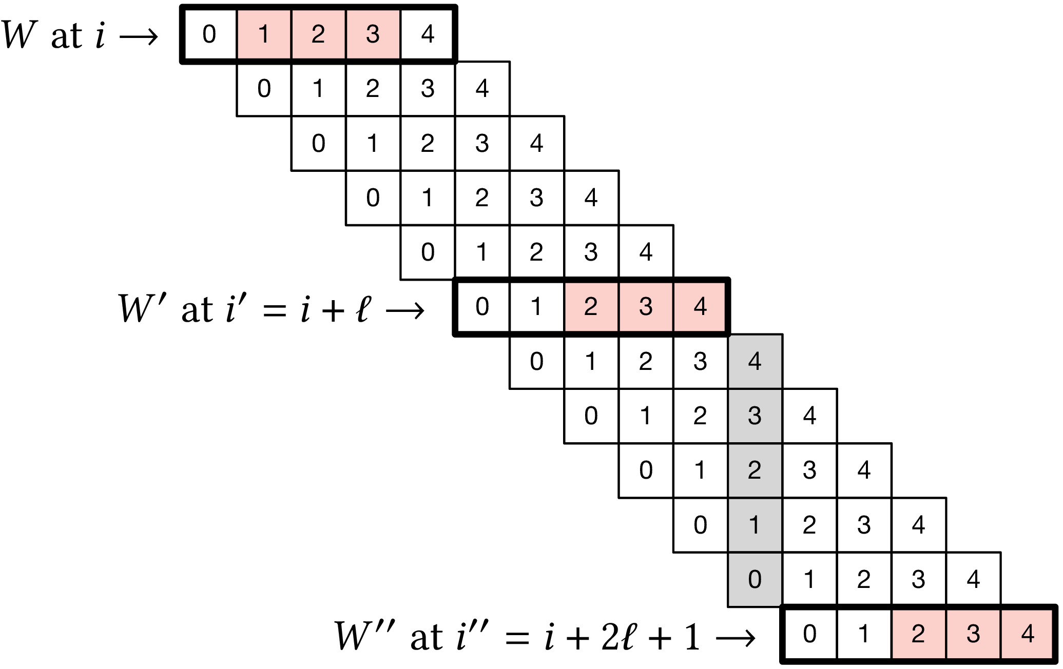
Figure 2: Setting used in proving the lower bound. In this example, we use (w=k=3), so (ell=w+k-1=5). Red boxes indicate the sampled (k)-mer in windows (W), (W’), and (W’’) that are highlighted with a ticker stroke.
We assume the input is an infinitely long random string \(S\) over \(\Sigma\). The proof makes use of the setting illustrated in Figure 2, which is as follows. We partition the windows of \(S\) in consecutive groups of \(2\ell+1\) windows. Let one such group of windows start at position \(i\), and consider windows \(W\) and \(W’\) starting at positions \(i\) and \(i’:= i+\ell\) respectively. Also let \(W’’\) be the window that is the exclusive end of the group, thus starting at position \(i’’ =i+2\ell+1 = i’+\ell+1\). Note that there is no gap between the end of window \(W\) and the beginning of window \(W’\), whereas there is a gap of a single character between the end of \(W’\) and the beginning of \(W’’\). (shown as the gray shaded area in Figure 2). These three windows are disjoint and hence the random variables \(X\), \(X’\), and \(X’’\) indicating \(f(W)\), \(f(W’)\), and \(f(W’’)\) respectively are independent and identically distributed. (But note that we do not assume they are uniformly distributed, as that depends on the choice of the sampling function \(f\).) In Figure 2, we have \(X=1\) and \(X’=X’’=2\).
Since the three windows \(W\), \(W’\), and \(W’’\) are disjoint, they sample \(k\)-mers at distinct positions. (indicated by the red boxes in Figure 2). The proof consists in computing a lower bound on the expected number of sampled \(k\)-mers in the range \([i+X, i’’+X’’)\). Note that for non-forward schemes, it is possible that windows before \(W\) or after \(W’’\) sample a \(k\)-mer inside this range. For our lower bound, we will simply ignore such sampled \(k\)-mers.
When \(X<X’\), the window starting at \(i+X+1\) ends at \(i+X+\ell = i’+X < i’+X’\), thus at least one additional \(k\)-mer must be sampled in the windows between \(W\) and \(W’\). Similarly, when \(X’ \leq X’’\), the window starting at \(i’+X’+1\) ends at \(i’ + X’ + \ell = i’’+X’-1 < i’’+X’’\), so that at least another \(k\)-mer must be sampled in the windows between \(W’\) and \(W’’\).
Thus, the number of sampled \(k\)-mers from position \(i+X\) (inclusive) to \(i’’+X’’\) (exclusive) is at least \({1+\pr[X < X’] + 1 + \pr[X’\leq X’’]}\). Since \(X\), \(X’\), and \(X’’\) are i.i.d., we have that \(\pr[X’\leq X’’] = \pr[X’\leq X] = 1 - \pr[X < X’]\), and hence \[ 1+\pr[X < X’] + 1 + \pr[X’\leq X’’] = 3. \] Since there are \(2\ell+1\) windows in each group, by linearity of expectation, we obtain density at least \[ \frac{3}{2\ell+1} = \frac{1.5}{w+k-0.5}. \]
This new version does not include the \(\max\left(0, \floor{\frac{k-w}{w}}\right)\) term, because it turns out that when \(k\geq w\), the full bound is anyway less than \(1/w\).
In Figure 3 we can see that this new version indeed provides a small improvement over the previous lower bound when \(k < (w+1)/2\). Nevertheless, a big gap remains between the lower bound and, say, the density of the random minimizer.
It is also clear that this proof is far from tight. It uses that an additional \(k\)-mer must be sampled when a full window of \(w+k-1\) characters fits between \(s_1\) and \(s_2\), while in practice an additional \(k\)-mer is already needed when the distance between them is larger than \(w\). However, exploiting this turns out to be difficult: we can not assume that the sampled positions in overlapping windows are independent, nor is it easy to analyse a probability such as \(\P[X \leq X’’-k]\).
2.4 A near-tight lower bound on the density of forward sampling schemes Link to heading
Together with Kille et al., in (Kille et al. 2024) we prove a nearly tight lower bound on the density of forward schemes. We start with a slightly simplified version.
Any forward scheme \(f\) has a density at least \[ d(f) \geq \frac{\ceil{\frac{w+k}{w}}}{w+k}. \]
The density of a forward scheme can be computed as the probability that two consecutive windows in a random length \(w+k\) context sample different \(k\)-mers (Lemma Marçais et al. 2017, 4). From this, it follows that we can also consider cyclic strings (cycles) of length \(w+k\), and compute the expected number of sampled \(k\)-mers along the cycle. The density is then this count divided by \(w+k\).
Because of the window guarantee, at least one out of every \(w\) \(k\)-mers along the length \(w+k\) cycle must be sampled. Thus, at least \(\lceil (w+k)/w\rceil\) \(k\)-mers must be sampled in each cycle. After dividing by the number of \(k\)-mers in the cycle, we get the result.
The full and more precise version is as follows (Theorem Kille et al. 2024, 1).
Let \(M_\sigma(p)\) count the number of aperiodic necklaces of length \(p\) over an alphabet of size \(\sigma\). Then, the density of any forward sampling scheme \(f\) is at least \[ d(f) \geq g_\sigma(w,k) := \frac{1}{\sigma^{w+k}} \sum_{p | (w+k)} M_\sigma(p) \left\lceil \frac pw\right\rceil \geq \frac{\left\lceil\frac{w+k}{w}\right\rceil}{w+k} \geq \frac 1w, \] where the middle inequality is strict when \(w>1\).
The core of this result is to refine the proof given above. While indeed we know that each cycle will have at least \(\ceil{(w+k)/w}\) sampled \(k\)-mers, that lower bound may not be tight. For example, if the cycle consists of only zeros, each window samples position \(i + f(000\dots 000)\), so that in the end every position is sampled.
We say that a cycle has period \(p\) when it consists of \((w+k)/p\) copies of some pattern \(P\) of length \(p\), and \(p\) is the maximum number for which this holds. In this case, we can consider the cyclic string of \(P\), on which we must sample at least \(\ceil{p/w}\) \(k\)-mers. Thus, at least \(\frac{w+k}{p}\ceil{\frac pw}\) \(k\)-mers are sampled in total, corresponding to a particular density along the cycle of at least \(\frac{1}{p}\ceil{\frac pw}\).
Since \(p\) is maximal, the pattern \(P\) itself must be aperiodic. When \(M_\sigma(p)\) counts the number of aperiodic cyclic strings of length \(p\), the probability that a uniform random cycle has period \(p\) is \(p\cdot M_\sigma(p) / \sigma^{w+k}\), where the multiplication by \(p\) accounts for the fact that each pattern \(P\) gives rise to \(p\) equivalent cycles that are simply rotations of each other. Thus, the overall density is simply the sum over all \(p\mid (w+k)\): \[ d(f) \geq \sum_{p | (w+k)} \frac{p\cdot M_\sigma(p)}{\sigma^{w+k}}\cdot \frac{1}{p} \left\lceil \frac pw\right\rceil =\frac 1{\sigma^{w+k}} \sum_{p | (w+k)} M_\sigma(p) \left\lceil \frac pw\right\rceil. \] The remaining inequalities follow by simple arithmetic.
As can be seen in Figure 3, this lower bound jumps up at values \(k\equiv 1 \pmod w\). In practice, if some density \(d\) can be achieved for parameters \((w,k)\), it can also be achieved for any larger \(k’\geq k\), by simply ignoring the last \(k’-k\) characters of each window. Thus, we can ‘‘smoothen’’ the plot via the following corollary.
Any forward scheme \(f\) has density at least \[ d(f) \geq g’_\sigma(w,k) := \max\big(g_\sigma(w,k), g_\sigma(w,k’)\big) \geq \max\left(\frac 1{w+k}\ceil{\frac{w+k}w}, \frac1{w+k’}\ceil{\frac{w+k’}w}\right), \] where \(k’\) is the smallest integer \(\geq k\) such that \(k’ \equiv 1 \pmod w\).
At this point, one might assume that a smooth ‘‘continuation’’ of this bound (that exactly goes through the ‘‘peaks’’) also holds, but this turns out to not be the case, as for example for \(\sigma=w=2\), the optimal scheme exactly follows the lower bound.
Local schemes. The lower bounds discussed so far can also be extended to local schemes by replacing \(c=w+k\) by \(c=2w+k-2\). Sadly, this does not lead to a good bound. In practice, the best local schemes appear to be only marginally better than the best forward schemes, while the currently established theory requires us to increase the context size significantly, thereby making all inequalities much more loose. Specifically, the tightness of the bound is mostly due to the rounding up in \(\frac{1}{c}\ceil{\frac{c}{k}}=\frac{1}{w+k}\ceil{\frac{w+k}{k}}\), and the more we increase \(c\), the smaller the effect of the rounding will be.
Searching optimal schemes. For small parameters \(\sigma\), \(w\), and \(k\), we can search for optimal schemes using an integer linear program (ILP) (Kille et al. 2024). In short, we define an integer variable \(x_W=f(W) \in [w]\) for every window \(W \in \sigma^{w+k-1}\), that indicates the position of the \(k\)-mer sampled from this window. For each context containing consecutive windows \(W\) and \(W’\), we add a boolean variable \(y_{(W, W’)}\) that indicates whether this context is charged. Additionally, we impose that \(f(W’) \geq f(W)-1\) to ensure the scheme is forward. The objective is to minimize the number of charged edges, i.e., to minimize the number of \(y\) that is true. In practice, the ILP can be sped up by imposing constraints equivalent to our lower bound: for every pure cycle of length at most \(w+k\), at least \(\ceil{(w+k)/w}\) of the contexts must be charged. This helps especially when \(k\equiv 1\pmod w\), in which case it turns out that the ILP always finds a forward scheme matching the lower bound, and hence can finish quickly.
2.5 Discussion Link to heading

Figure 3: Comparison of forward scheme lower bounds and optimal densities for small (w), (k), and (sigma). Optimal densities were obtained via ILP and are shown as black circles that are solid when their density matches the lower bound (g’_sigma), and hollow otherwise. Each column corresponds to a parameter being fixed to the lowest non-trivial value, i.e., (sigma=2) in the first column, (w=2) in the second column, and (k=1) in the third columns. Note that the x-axis in the third column corresponds to (w), not (k). This figure appeared before in (Kille et al. 2024) and was made in collaboration with Bryce Kille. The ILP implementation is also his.
In Figure 3 we compare the lower bounds to optimal schemes for small parameters. First, note that the bound of Marçais et al. (grey) is only better than \(1/w\) for small \(k<(w+1)/2\). In this regime, the improved version (green) indeed gives a slight improvement. The simple version of the near-tight bound (blue) is significantly better, and closely approximates the best ILP solutions when at least one of the parameters is large enough. When all parameters are small, the improved version \(g_\sigma\) (purple) is somewhat better though. As discussed, the density can only decrease in \(k\), and indeed the monotone version \(g’_\sigma\) (red) is much better.
We see that the bound exactly matches the best forward scheme when \(k=1\) and the ILP succeeded to find a solution (third column), and more generally when \(k\equiv 1\pmod w\). Furthermore, for \(\sigma=w=2\), the lower bound is also optimal for all even \(k\). Thus, we have the following open problem.
Prove that the \(g’_\sigma\) lower bound on forward scheme density is tight when \(k\equiv 1\pmod w\), and additionally when \(\sigma=w=2\).
For the remaining \(k\), specifically \(1<k<w\), there is a gap between the lower bound and the optimal schemes.
Can we find a ‘‘clean’’ proof of a lower bound on forward scheme density that matches the optimal schemes for \(1<k<w\), or more generally when \(k\not\equiv 1\pmod w\)?
And lastly, a lot is still unknown about local schemes.
In practice, local schemes are only slightly better than forward schemes, while the current best lower-bounds for local schemes are much worse. Can we prove a lower bound that is close to that of forward schemes? Or can we bound the improvement that local schemes can make over forward schemes?
Commentary. Bryce Kille and myself independently discovered the basis of the tight lower bound during the summer of 2024. In hindsight, I am very surprised it took this long (over 20 years!) for this theorem to be found. Minimizers were originally defined in 2003-2004, and only in 2018 the first improvement (or fix, rather) of Schleimer et al.’s original bound was found by Marçais et al. (Marçais, DeBlasio, and Kingsford 2018). Specifically, all ingredients for the proof have been around for quite some time already:
- The density of the random minimizer is \(2/(w+1)\), which ‘‘clearly’’ states: out of every \(w+1\) consecutive \(k\)-mers, at least \(2\) must be sampled. We just have to put those characters into a cycle.
- The density of any forward scheme can be computed using an order \(w+k\) De Bruijn sequence, so again, it is only natural that looking at strings of length at least \(w+k\) is necessary. Cyclic strings are a simple next step.
- And also, partitioning the De Bruijn graph into cycles is something that was done before by Mykkeltveit (Mykkeltveit 1972).
3 Practical Sampling Schemes Link to heading
In this chapter, we review existing minimizer schemes and more general sampling schemes. They fall into a few categories: they are variants of lexicographic minimizers, based on universal hitting sets with a greedy construction, or based on syncmers.
We then introduce the open-closed minimizer (Groot Koerkamp, Liu, and Pibiri 2025), which is a small variant of miniception that not only uses closed syncmers, but also open syncmers. Then, we introduce the (extended) mod-minimizer (Groot Koerkamp and Pibiri 2024), which is a practical minimizer scheme that reaches asymptotic optimal density \(1/w\) as \(k\to\infty\). For large alphabets, the mod-minimizer exactly matches the density of the lower bound when \(k\equiv 1\pmod w\). Together, these make the mod-minimizer the lowest density scheme when \(k>w\).
This chapter is based on two papers. ‘‘The mod-minimizer: A simple and efficient sampling algorithm for long \(k\)-mers’’ (Groot Koerkamp and Pibiri 2024) is coauthored with Giulio Ermanno Pibiri and introduces the mod minimizer. The followup paper ‘‘The open-closed mod-minimizer algorithm’’ (Groot Koerkamp, Liu, and Pibiri 2025) was written with Giulio Ermanno Pibiri and Daniel Liu and introduces the open-closed minimizer and the extended mod-minimizer.
The idea for the mod-minimizer is my own. The open-closed minimizer was found in close collaboration with Daniel Liu and Giulio Ermanno Pibiri. For both papers, the implementation, evaluation, and writing of the paper were done in equal parts by Giulio Ermanno Pibiri and myself.
We now turn our attention from lower bounds and towards low-density sampling schemes. We first consider various existing schemes, that we go over in three groups. In Section 3.1 we consider some simple variants of lexicographic minimizers. In Section 3.2, we consider some schemes that build on universal hitting sets, either by explicitly constructing one or by using related theory. We also include here the greedy minimizer, which is also explicitly constructed using a brute force search. Then, in Section 3.3, we cover some schemes based on syncmers.
We end with two new schemes. First, the open-closed minimizer (Groot Koerkamp, Liu, and Pibiri 2025) (Section 3.4), which extends the miniception by first preferring the smallest open syncmer, falling back to the smallest closed syncmer, and then falling back to the smallest \(k\)-mer overall. This simple scheme achieves near-best density for \(k\leq w\).
Second, we introduce the (extended) mod-minimizer and the open-closed mod-mini (Groot Koerkamp and Pibiri 2024; Groot Koerkamp, Liu, and Pibiri 2025). These schemes significantly improve over all other schemes when \(k>w\) and converge to density \(1/w\) as \(k\to\infty\). Additionally, we show that they have optimal density when \(k\equiv 1\pmod w\) and the alphabet is large.
3.1 Variants of lexicographic minimizers Link to heading
The lexicographic minimizer is known to have relatively bad density because it
is prone to sampling multiple consecutive \(k\)-mers when there is a run of A characters.
Nevertheless, they achieve density \(O(1/w)\) as \(k=\floor{\log_\sigma(w/2)}-2\)
and \(w\to\infty\) (Zheng, Kingsford, and Marçais 2020).
They can be improved by using an slightly modified order (Roberts et al. 2004):
The alternating order compares \(k\)-mers by by using lexicographic order for
characters in even positions (starting at position \(0\)), and reverse
lexicographic order for all odd positions. Thus, the
smallest string is be AZAZAZ....
This scheme typically avoids sampling long runs of equal characters, unless the entire window consists only of a single character.
A second variant is the ABB order (Frith, Noé, and Kucherov 2020).
The ABB order compares the first character lexicographically, and then uses order
B = C = ... = Z < A from the second position onward, so that the smallest string is ABBBB...,
where the number of non-A characters following the first A is maximized.
This scheme has the property that distinct occurrences of the ABB...
pattern are necessarily disjoint, leading to good spacing of the minimizers.
This was already observed before in the context of generating non-overlapping
codes (Blackburn 2015).
A drawback of the ABB order is that it throws away some information: for example
AB and AC are considered equal, which is usually not idea. Thus, we also
consider a version with tiebreaking, ABB+:
The ABB+ order first compares two \(k\)-mers via the ABB order, and in case of a tie, compares them via the plain lexicographic order.
We also introduce a small variation on these schemes.
The anti-lexicographic order sorts \(k\)-mers by comparing the first character lexicographically, and comparing all remaining characters reverse lexicographically.
In this order, the smallest string is AZZZZ....
Evaluation Link to heading

Figure 4: Comparison of the density of variants of lexicographic minimizers, for alphabet size (sigma=4), (w=24), and varying (k). The (g’) lower bound is shown in red and the trivial (1/w) lower bound in shown in black. The solid lines indicate the best density up to (k), which for the random minimizer happens to be best for (k=4) due to the selected random hash function. ABB+ indicates the ABB order with lexicographic tiebreaking.
In Figure 4, we compare the aforementioned variants of lexicographic minimizers. First, note that all schemes perform bad for \(k\in \{1,2\}\), since \(k^\sigma\leq 2^4=16 < 24=w\), and thus there will always be duplicate \(k\)-mers. As expected, the random minimizer (yellow) has density \(0.08 = 2/(24+1)\). The lexicographic order (dim blue) is significantly worse at 0.89. The alternating order (orange, 0.78) is slightly better, and the anti-lex order (green, 0.76) is slightly better again.
The ABB order (red-purple, 0.69), and especially the ABB order with tiebreaking (blue) perform much better than the random minimizer. ABB+tiebreaking even performs nearly optimal for \(3\leq k\leq 5\). This is surprising, since the idea was already introduced as a sampling and minimizer scheme in 2020 (Fig Frith, Noé, and Kucherov 2020, 4 a) and appeared more generally before in 2015, but somehow never was compared against by other minimizer schemes. In particular, as we will see later, this scheme outperforms most other schemes for small \(k\), and e.g. miniception (also 2020) is only slightly better for large \(k\).
3.2 UHS-inspired schemes Link to heading
We first have a look at minimizer schemes that build on universal hitting sets. Of these schemes, all but the decycling minimizer use a bruteforce search to search small universal hitting sets, or minimizers schemes directly for GreedyMini. This means that those schemes are limited to cases where \(k\) and \(w\) are sufficiently small that this bruteforce search can finish in reasonable time. For DOCKS, \(\boldremuval\), and PASHA, (double) decycling is better in practice, and thus we omit them from comparisons.
DOCKS. Orenstein et al. (Orenstein et al. 2016, 2017) introduce an algorithm to generate small universal hitting sets. It works in two steps. It starts by using Mykkeltveit’s minimum decycling set (Mykkeltveit 1972) such that every infinitely long string contains a \(k\)-mer from the decycling set. Then, it repeatedly adds the \(k\)-mer to the UHS that is contained in the largest number of length \(\ell=w+k-1\) windows that does not yet contain a \(k\)-mer in the UHS. In practice, the exponential runtime in \(k\) and \(w\) is a bottleneck. A first speedup is to consider the \(k\)-mer contained in the largest number of paths of any length. A second method for larger \(k’ > k\), called naive extension, is to simply ignore the last \(k’-k\) characters of each \(k\)-mer and then use a UHS for \(k\)-mers. DOCKS can generate UHSes up to around \(k=13\), and for \(k=10\) and \(w=10\), it has density down to \(1.737/(w+1)\) (Marçais et al. 2017), thereby being the first scheme that breaks the conjectured \(2/(w+1)\) lower bound.
\(\boldremuval\) (DeBlasio et al. 2019) is a method that builds on DOCKS. Starting with some \((w,k-1)\) UHS generated by DOCKS, first uses naive extension to get a \((w, k)\) UHS \(U’\). Then, it tries to reduce the size of this new UHS by removing some \(k\)-mers. In particular, if a \(k\)-mer only ever occurs in windows together with another \(k\)-mer of \(U’\), then this \(k\)-mer may be removed from \(U’\). Instead of greedily dropping \(k\)-mers, and ILP is built to determine an optimal set of \(k\)-mers to drop. This process is repeated until the target \(k\) is reached, which can be up to at least \(200\), as long as \(w\leq 21\) is sufficiently small.
PASHA (Ekim, Berger, and Orenstein 2020) also builds on DOCKS and focuses on improving the construction speed. It does this by parallellizing the search for \(k\)-mers to add to the UHS, and by adding multiple \(k\)-mers at once (each with some probability) rather than only the one with the highest count of un-covered windows containing it. These optimizations enable PASHA to generate schemes up to \(k=16\), while having density comparable to DOCKS.
Decycling-based minimizer. An improvement to the brute force constructions of DOCKS, \(\remuval\), and PASHA came with a minimizer scheme based directly on minimum decycling sets (Pellow et al. 2023): In any window, prefer choosing a \(k\)-mer in \(\Dk\), if there is one, and break ties using a random order. They also introduce the double decycling scheme. This uses the symmetric MDS \(\Dtk\) consisting of those \(k\)-mers for which \(-2\pi/k\leq \arg(x)<0\). It then first prefers \(k\)-mers in \(\Dk\), followed by \(k\)-mers in \(\Dtk\), followed by \(k\)-mers that are in neither.
It is easy to detect whether a \(k\)-mer is in the MDS or not without any memory, so that this method scales to large \(k\). Surprisingly, not only is this scheme conceptually simpler, but it also has significantly lower density than DOCKS, PASHA, and miniception. Apparently, the simple greedy approach of preferring smaller \(k\)-mers works better than the earlier brute force searches for small universal hitting sets. Especially for \(k\) just below \(w\), its density is much better than any other scheme.
GreedyMini. Unlike the previous UHS schemes, GreedyMini (Golan et al. 2025) directly constructs a low-density minimizer scheme using a brute force approach. As we saw, the density of a minimizer scheme equals the probability that the smallest \(k\)-mer in a \(w+k\) long context is at the start or end. The GreedyMini builds a minimizer scheme by one-by-one selecting the next-smallest \(k\)-mer. It starts with the set of all \(w+k\) contexts, and finds the \(k\)-mer for which the number of times it appears as the first or last \(k\)-mer in a context, as a fraction of its total number of appearances, is lowest. It then discards all contexts this \(k\)-mer appears in, and repeats the process until a minimizer has been determined for all contexts. To improve the final density, slightly submoptimal choices are also tried occasionally, and a local search and random restarts are used. To keep the running time manageable, the schemes are only built for a \(\sigma=2\) binary alphabet and up to \(k\leq 20\). This is extended to larger \(k\) using naive extension and to larger alphabets by simply ignoring some of the input bits.
The resulting schemes achieve density very close to the lower bound, especially when \(k\) is around \(w\). In these regions, the greedymini has lower density than all other schemes, and it is able to find optimal schemes for some small cases when \(k\equiv 1\pmod w\). This raises the question whether it is also optimal for other \(k\), where the lower bound may not be tight yet. A drawback is that this scheme is not pure: it must explicitly store the chosen order of \(k\)-mers. In particular, our choice of \(w=24\) is much larger than the parameters for which precomputed schemes are provided, and so we omit it from the comparison in Figure 5.
3.3 Syncmer-based schemes Link to heading
As we saw, universal hitting sets belong to a more general class of context-free schemes that only look at individual \(k\)-mers to decide whether or not to sample them. A well-known category of context-free schemes are syncmers (Edgar 2021). In general, syncmer variants consider the position of the smallest \(s\)-mer inside a \(k\)-mer, for some \(1\leq s\leq k\) and according to some order \(\Os\). Here we consider two well-known variants: closed and open syncmers.
A \(k\)-mer is a closed syncmer when the (leftmost) smallest contained \(s\)-mer according to some order \(\Os\), is either the first \(s\)-mer at position \(0\) or the last \(s\)-mer at position \(k-s\).
Closed syncmers satisfy a window guarantee of \(k-s\), meaning that there is at least one closed syncmer in any window of \(w\geq k-s\) consecutive \(k\)-mers. When the order \(\Os\) is random, closed syncmers have a density of \(2/(k-s+1)\), which is the same as that of a random minimizer when \(k>w\) and \(s=k-w\). Indeed, syncmers were designed to improve the conservation metric rather than the density. See the paper by Edgar (Edgar 2021) for details.
A \(k\)-mer is an open syncmer whe the smallest contained \(s\)-mer (according to \(\Os\)) is at a specific offset \(v\in [k-s+1]\). In practice, we always use \(v = \floor{(k-s)/2}\).
The choice of \(v\) to be in the middle was shown to be optimal for conservation (Shaw and Yu 2021). For this \(v\), open syncmers satisfy a distance guarantee (unlike closed syncmers): two consecutive open syncmers are always at least \(\floor{(k-s)/2}+1\) positions apart.
Miniception is a minimizer scheme that builds on top of closed syncmers (Zheng, Kingsford, and Marçais 2020). The name stands for ‘‘minimizer inception’’, in that it first uses an order \(\Os\) and then an order \(\Ok\).
Let \(w\), \(k\), and \(s\) be given parameters and \(\Ok\) and \(\Os\) be orders. Given a window \(W\) of \(w\) \(k\)-mers, miniception samples the smallest closed syncmer if there is one. Otherwise, it samples the smallest \(k\)-mer.
Because of the window guarantee of closed syncmers, miniception always samples a closed syncmer when \(w\geq k-s\). When \(k\) is sufficiently larger than \(w\) and \(s = k-w+1\), it is shown that miniception has density bounded by \(1.67/w + o(1/w)\). In practice, we usually use \(s = k-w\) when \(k\) is large enough. Unlike UHS-based schemes, miniception does not require large memory, and it is the first such scheme that improves the \(2/(w+1)\) density when \(k\approx w\).
3.4 Open-closed minimizer Link to heading
As we saw, Miniception samples the smallest \(k\)-mer that is a closed syncmer. The open-closed minimizer is a natural extension of this (Groot Koerkamp, Liu, and Pibiri 2025):
Given parameters \(w\), \(k\), and \(1\leq s\leq k\), and orders \(\Ok\) and \(\Os\), the open-closed minimizer samples the smallest (by \(\Ok\)) \(k\)-mer in a window that is an open syncmer (by \(\Os\)), if there is one. Otherwise, it samples the smallest \(k\)-mer that is a closed syncmer. If also no closed syncmer is present, the overall smallest \(k\)-mer is sampled.
The rationale behind this method is that open syncmers have a distance lower bound (Edgar 2021), i.e., any two open syncmers are at least \(\floor{(k-s)/2}+1\) positions apart. This is in contrast to closed syncmers, that do not obey a similar guarantee (but instead have an upper bound on the distance between them). As it turns out, by looking at Figure 5, the distance lower bound of open syncmers (O, red-purple) gives rise to lower densities than the upper bound of closed syncmers (C=miniception, green).
In the full paper (Groot Koerkamp, Liu, and Pibiri 2025), we give a polynomial algorithm to compute the exact density of the open-closed minimizer scheme, assuming that no duplicate \(k\)-mers occur. At a high level, this works by considering the position of the smallest \(s\)-mer in the window, and then recursing on the prefix or suffix before/after it, until an \(s\)-mer is found that is sufficiently far from the boundaries to induce an open syncmer.
Evaluation Link to heading

Figure 5: Comparison of the density of pure minimizer schemes, for alphabet size (sigma=4), (w=24), and varying (k). The solid lines indicate the best density up to (k). The open-closed minimizer has the OC label, and the O and C labels correspond to preferring open or closed syncmers before falling back to a random order. We use (s=4) for the syncmer-based schemes.
In Figure 5, we compare all pure schemes seen so far. We see that miniception (green) performs slightly better than the ABB+tiebreak order when \(k\) is sufficiently large. The decycling-set based orders (grey and black) significantly outperform the miniception, especially for \(k\) just below \(w\). Surprisingly, just changing the closed syncmers of miniception for open syncmers (O, red-purple) yields a better scheme, although not as good as decycling. The combination (OC, purple) does reach the same density as double decycling, and improves over it for \(w\leq k\leq 2w\). Interestingly, the O and OC curves look similar to the decycling and double decycling curves, but slightly shifted to the right. The right shift is caused by looking at syncmers where the inner minimizer has length \(s=4\). If we were to use a large alphabet with \(s=1\), this difference mostly disappears.
3.5 Mod-minimizer Link to heading
So far, all the schemes we have seen in this section work well up to around \(k\approx w\), but then fail to further decrease in density as \(k\) grows to infinity. The rot-minimizer (Marçais, DeBlasio, and Kingsford 2018) does converge to density \(1/w\), but in its original form it only does so very slowly.
Here we present the mod-minimizer (Groot Koerkamp and Pibiri 2024; Groot Koerkamp, Liu, and Pibiri 2025), which turns out to converge to \(1/w\) nearly as fast as the lower bound we showed before in 2.
We start with a slightly more general definition.
Let \(W\) be a window of \(w+k-1\) characters, let \(1\leq t\leq k\) be a parameter, and let \(\Ot\) be a total order on \(t\)-mers. Let \(x\) be the position of the smallest \(t\)-mer in the window according to \(\Ot\). Then, mod-sampling samples the \(k\)-mer at position \(x \bmod w\).
As it turns out, this scheme is only forward for some choices of \(t\) (Lemma Groot Koerkamp and Pibiri 2024, 8).
Mod-sampling is forward if and only if \(t\equiv k\pmod w\) or \(t\equiv k+1\pmod w\).
Consider two consecutive windows \(W\) and \(W’\). Let \(x\) be the position of the smallest \(t\)-mer in window \(W\) and \(x’\) that of the smallest \(t\)-mer in \(W’\). mod-sampling is forward when \((x \bmod w) - 1 \leq (x’ \bmod w)\) holds for all \(x\) and \(x’\). Given that the two windows are consecutive, this trivially holds when \(x=0\) and when \(x’ = x-1\). Thus, the only position \(x’\) that could violate the forwardness condition is when \(W’\) introduces a new smallest \(t\)-mer at position \(x’=w+k-t-1\). In this case, we have \(x’ \bmod w = (w+k-t-1) \bmod w = (k-t-1) \bmod w\). The rightmost possible position of the sampled \(k\)-mer in \(W\) is \(x\bmod w = w-1\). Hence, if the scheme is forward, then it must hold that \((w-1)-1=w-2\leq(k-t-1) \bmod w\). Vice versa, if \(w-2\leq(k-t-1) \bmod w\) always holds true, then the scheme is forward. % since \(x \bmod w \leq w-1\).
Now, note that \((k-t-1) \bmod w \geq w-2 \iff qw-2 \leq k-t-1 < qw \iff k-qw \leq t \leq k-qw+1\) for some \(0 \leq q \leq \lfloor k/w \rfloor\). In conclusion, the scheme is forward if and only if \(t=k-qw\) or \(t=k-qw+1\), i.e., when \(t \equiv k \pmod w\) or \(t \equiv k+1 \pmod w\).

Figure 6: The density of the random minimizer and mod-sampling for varying (t), for (w=24) and (k=60). The random mod-minimizer has local minima in the density at (t=12) and (t=36), where (tequiv kequiv 12pmod w). There is also a local minimum at (t=3), which is the first (t) that is large enough to avoid duplicate (k)-mers. Based on this, we choose (t) to be the least number at least some lower bound (r) that satisfies (tequiv kpmod w). This figure is based on Figure 4 of (Groot Koerkamp and Pibiri 2024) which was made by Giulio Ermanno Pibiri.
In Figure 6, it can be seen that mod-sampling has local minima in the density when \(t\equiv k\pmod w\) (Lemma Groot Koerkamp and Pibiri 2024, 12), thus, we restrict our attention to this case only.
Furthermore, we can show that for \(t\equiv k \pmod w\), mod-sampling is not only forward, but also a minimizer scheme (Lemma Groot Koerkamp and Pibiri 2024, 13):
Mod-sampling is a minimizer scheme when \(t\equiv k\pmod w\).
Our proof strategy explicitly defines an order \(\order_k\) and shows that mod-sampling with \(t \equiv k \pmod w\) corresponds to a minimizer scheme using \(\order_k\), i.e., the \(k\)-mer sampled by mod-sampling is the leftmost smallest \(k\)-mer according to \(\order_k\).
Let \(\order_t\) be the order on \(t\)-mers used by mod-sampling Define the order \(\order_k(K)\) of the \(k\)-mer \(K\) as the order of its smallest \(t\)-mer, chosen among the \(t\)-mers occurring in positions that are a multiple of \(w\): \[ \order_k(K) = \min_{i \in \{0,w, 2w,\dots, k-t\}} \order_t(K[i..i+t)) \] where \(k-t\) is indeed a multiple of \(w\) since \(t\equiv k\pmod w\). Now consider a window \(W\) of consecutive \(k\)-mers \(K_0,\ldots,K_{w-1}\). Since each \(k\)-mer starts at a different position in \(W\), \(\order_k(K_i)\) considers different sets of positions relative to \(W\) than \(\order_k(K_j)\) for all \(i \neq j\). However, \(t\)-mers starting at different positions in \(W\) could be identical, i.e., the smallest \(t\)-mer of \(K_i\) could be identical to that of \(K_j\). In case of ties, \(\order_k\) considers the \(k\)-mer containing the leftmost occurrence of the \(t\)-mer to be smaller.
Suppose the leftmost smallest \(t\)-mer is at position \(x \in [w+k-t]\). Then mod-sampling samples the \(k\)-mer \(K_p\) at position \(p = x \bmod w\). We want to show that \(K_p\) is the leftmost smallest \(k\)-mer according to \(\order_k\). If \(\order_t(W[x..x+t))=o\), then
\begin{align*} \order_k(K_p) = \order_k(W[p..p+k)) &= \min_{j\in \{0,w, 2w,\dots, k-t\}} \order_t(W[p+j..p+j+t)) \\ &= \min_{j\in \{x-p\}} \order_t(W[p+j..p+j+t)) = o. \end{align*}
Since \(o\) is minimal, any other \(k\)-mer \(K_j\) must have order \(\geq o\). Also, since \(o\) is the order of the leftmost occurrence of the smallest \(t\)-mer, \(K_p\) is the leftmost smallest \(k\)-mer according to \(\order_k\).
This now allows us to define the mod-minimizer.
Let \(r = O(\log_\sigma(w))\) be a small integer lower bound on \(t\). For any \(k\geq r\), choosing \(t= r+((k-r)\bmod w)\) in combination with a uniform random order \(\Ot\) gives the mod-minimizer.
It turns out this definition can be extended to wrap any sampling scheme, rather than just random minimizers (Groot Koerkamp, Liu, and Pibiri 2025).
Let \(w\), \(k\), and \(t\equiv k\pmod w\) be given parameters, and let \(f: \Sigma^{w+k-1} \to [w+k-t]\) be any sampling scheme with parameters \((w’, k’) = (w+k-t, t)\). Then, given a window \(W\) of length \(w+k-1\), the extended mod-minimizer of \(f\) samples position \(f(W)\bmod w\).
Naturally, the extended mod-minimizer can be applied to the open-closed minimizer, to obtain the oc-mod-mini.
Theoretical density Link to heading
When we restrict \(f\) to be a minimizer scheme specifically, we can compute the density of the extended mod-minimizer (Theorem Groot Koerkamp, Liu, and Pibiri 2025, 1).
Let \(w\), \(k\), and \(t\equiv k\pmod w\) be given parameters, and let \(f\) be a minimizer scheme on \(t\)-mers with order \(\Ot\). Then, the density of the extended mod-minimizer is given by the probability that, in a context of length \(w+k\), the smallest \(t\)-mer is at a position \(0\pmod w\).
Consider two consecutive windows \(W\) and \(W’\) of length \(w+k-1\) of a uniform random string. Let \(x\) and \(x’\) be the position of the smallest \(t\)-mer in \(W\) and \(W’\) respectively, and let \(p=x\bmod w\) and \(p’=x’\bmod w\) be the positions of the sampled \(k\)-mers Let \(y\in\{x, x’+1\}\) be the absolute position of the smallest \(t\)-mer in the two windows.
Since \(A\) is a forward scheme, we can compute its density as the probability that a different \(k\)-mer is sampled from \(W\) and \(W’\). First note that the two consecutive windows contain a total of \(w+k-t+1\) \(t\)-mers, and thus, \(0\leq y\leq w+k-t\), where \(w+k-t\) is divisible by \(w\) since \(t\equiv k\pmod w\).
When \(y\not\equiv 0\pmod w\), this implies \(0<y<w+k-t\), and thus, the two windows share their smallest \(t\)-mer. Thus, \(p=x\bmod w = y\bmod w\) and \(p’+1=x’\bmod w+1=(y-1)\bmod w+1\). Since \(y\not\equiv 0\pmod w\), this gives \(p’+1=y\bmod w\), and thus, the two windows sample the same \(k\)-mer.
When \(y\equiv 0\pmod w\), there are two cases. When \(y=x\) (and thus \(y<w+k-t\)), we have \(p=x\bmod w=y\bmod w=0\), and since the \(k\)-mer starting at position \(0\) is not part of \(W’\), the second window must necessarily sample a new \(k\)-mer. Otherwise, we must have \(y=(x’+1)\equiv 0\pmod w\), which implies \(p’=x’\bmod w=(y-1)\bmod w=w-1\), and since the \(k\)-mer starting at position \(w-1\) in \(W’\) is not part of \(W\), again the second window must necessarily sample a new \(k\)-mer.
To conclude, the two windows sample distinct \(k\)-mer if and only if the smallest \(t\)-mer occurs in a position \(y\equiv 0\pmod w\).
Before we compute the density of the mod-minimizer, we first re-state Lemma 9 of (Groot Koerkamp and Pibiri 2024), which is a slightly modified version of Lemma 9 of (Zheng, Kingsford, and Marçais 2020) that we saw earlier in Section 1.7. The proof is nearly identical.
For any \(\varepsilon > 0\), if \(t > (3+\varepsilon) \log_\sigma(\ell)\), the probability that a random window of \(\ell-t+1\) \(t\)-mers contains two identical \(t\)-mers is \(o(1/\ell)\). Given that \(\ell = w+k-1\), \(o(1/\ell) \to 0\) for \(k\to\infty\).
From the above two results, we obtain the density of the random mod-minimizer (Corollary Groot Koerkamp and Pibiri 2024, 17)(Theorem Groot Koerkamp, Liu, and Pibiri 2025, 2).
If \(t\equiv k\pmod w\) satisfies \(t > (3+\varepsilon) \log_\sigma(\ell)\) for some \(\varepsilon > 0\), the density of the random mod-minimizer is \[ \frac{2+\frac{k-t}{w}}{w+k-t+1} + o(1/(w+k-1)). \] When \(w\) is fixed and \(k\to\infty\), this density tends to \(1/w\).
Given the bound on \(t\), the probability that a context of \(w+k\) characters contains duplicate \(t\)-mers is \(o(1/\ell) = o(1/(w+k-1))\). Otherwise, the context contains \(w+k-t+1\) \(t\)-mers, of which the ones at positions \(\{0, w, 2w, \dots, w+k-t\}\) cause the context to be charged, which is a fraction of \(\frac{2+\frac{k-t}{w}}{w+k-t+1}\) of all \(t\)-mers.
The random mod-minimizer has optimal density when \(w\) is fixed, \(r=t=1\), \(k\equiv 1\pmod w\), and \(\sigma\to\infty\).
First note that the probability of duplicate \(k\)-mers in a window goes to \(0\) as \(\sigma\to\infty\), and hence the error term in the density computed above disappears. Substituting variables, we get \[ \frac{2+\lfloor\frac{k-1}{w}\rfloor}{w+\lfloor\frac{k-1}{w}\rfloor w+1} = \frac{2+\frac{k-1}{w}}{w+\frac{k-1}{w} w+1} = \frac{\frac{k+2w-1}w}{k+w} = \frac{\lceil\frac{k+w}w\rceil}{k+w}. \]
Evaluation Link to heading

Figure 7: Comparison of the density of extended mod-minimizer schemes, for alphabet size (sigma=4), (w=24), (r=4), and varying (k). The solid lines indicate the best density up to (k). Versions without mod-mini are shown dimmed.
In Figure 7, we compare the mod-minimizer version of the best schemes so far against their normal density. We use \(r=4\) as the lower bound on \(t\), so that repeated \(t\)-mers are rare in practice. We clearly see that the mod-minimizer schemes roughly follow the red lower bound, and indeed have density that converges to \(1/w\) as \(k\) increases. Between \(k=w+1\) and \(k=2w+1\), the graphs look roughly similar to the area between \(k=1\) and \(k=w+1\): ABB with tiebreaking is best when \(k\) is small (up to around \(w/2\)), and hence also when \(t\) is small (again up to around \(w/2\)). For larger \(k\) and \(t\), we see that double decycling has minimal density.
Like the OC-minimizer, the mod-minimizer requires \(t\geq 4\) to avoid duplicate \(k\)-mers. This causes the graphs to jump down at \(k=w+4\), rather than at \(k=w+1\). When the alphabet is large, \(t=1\) suffices, and the graphs of the mod-minimizer touch lower bound when \(k\equiv 1\pmod w\).
3.6 Discussion Link to heading
Looking at Figure 7, there are still some regions where we do not yet have near-optimal sampling schemes. First, when \(k \leq 2\), all schemes have poor density, as minimizer schemes generally can not do well when \(k\leq \log_\sigma(w)\) (Theorem 17). In the next section, we will investigate forward schemes that do achieve good density for such small \(k\).
Secondly, when \(\sigma=4\) and \(k\leq w\) or slightly smaller, the current schemes do not achieve near-optimal density, while we do expect such schemes to exist based on the ILP results for small parameters. Indeed, the greedy minimizer appears to be near-optimal for \(k\) close to \(w\). Nevertheless, for roughly \(w/6 < k < \frac 23 w\), no schemes are close to the lower bound, and specifically at \(k = w/3\), the ‘‘deepest’’ point of the lower bound, the gap is large.
Is there a pure forward sampling scheme with density close or equal to the lower bound \(g’_\sigma\) for \(k\approx w\) or \(k\approx w/3\)? Is it possible when \(\sigma\to\infty\)? Or when \(w\to\infty\)?
4 Towards Optimal Selection Schemes Link to heading
We end this part on minimizers with a look into selection schemes, which are sampling schemes with \(k=1\). These are interesting, because the lower bound appears to be tight: for small parameters, the brute force search finds exactly optimal schemes. Thus, we ask ourselves whether we can construct ‘‘pure’’ optimal schemes that are simple to understand and analyze.
We first review bidirectional anchors (bd-anchors) (Loukides and Pissis 2021). Then, we newly introduce smallest-unique-substring anchors, or sus-anchors. Initially these improve only slightly over bd-anchors, and by changing from lexicographic order to anti-lexicographic order, they become nearly optimal.
We end with a discussion on the remaining gap between our scheme and the true lower bound, and how this could be closed. More generally, we also recap the results on minimizer density we obtained, and state some open problems related to this.
This chapter is based on unpublished notes that are my own work. Some of the open problems in the discussion are based on previously written discussions (Groot Koerkamp and Pibiri 2024; Groot Koerkamp, Liu, and Pibiri 2025; Kille et al. 2024).
[By now, a preprint on the anti-lexicographic SUS-anchor is Groot Koerkamp (2026).]
As we saw for the sampling schemes so far, they do not do well for very small \(k\). Indeed, they are all minimizer schemes, and these can not achieve density below \(1/\sigma^k\). More generally, when \(w\to\infty\), any fixed finite \(k\) at some point becomes less than \(\log_\sigma(w)\) and thus too small to result in a good minimizer scheme. At that point, we instead have to consider more general sampling schemes to still be able to achieve density close to the lower bound. Here, we take this to the limit and explore the \(k=1\) case, which are also called selection schemes. In this case, the window size is \(\ell=w+k-1=w\), and thus, the task is to select any of the \(w\) characters in a window of length \(w\).
We first introduce bidirectional anchors (Loukides and Pissis 2021) in 4.1, and then we improve these into smallest-unique-substring anchors in 4.2, which is unpublished work of myself.
4.1 Bidirectional anchors Link to heading
Bidirectional anchors (bd-anchors) are a variant on minimizers that take the minimal lexicographic rotation instead of the minimal \(k\)-mer substring (Loukides and Pissis 2021):
Given a window \(W\) of length \(w\), the bidirectional anchor is the lexicographical minimal rotation of the window, starting at position \(i\in [w]\), so that \(W[i, w)W[0, i) \leq W[j, w)W[0, j)\) for all \(j\). In case of ties, the leftmost minimal rotation is chosen.
It turns out that bd-anchors are somewhat brittle because the are not forward:
for example, take the window
ZABAAC, that has minimal rotation starting with AAC.... If we then shift the
window by one, we may get ABAACA, of which the smallest rotation AAB...
starts at the end. Shifting again to e.g. BAACAY, the smallest rotation again
starts with AAC.... Thus, in the middle step, the final A was only sampled
because the string happened to start with an A as well at that single step.
Reduced bd-anchors solve this, although they are still not forward
(Definition Loukides, Pissis, and Sweering 2023, 2).
Given a parameter \(0\leq r< w\), the reduced bidirectional anchor of a window \(W\) of length \(w\) is the lexicographic smallest rotation starting at a position \(i\in [w-r]\).
Now, the following theorem can be proven (Lemma Loukides, Pissis, and Sweering 2023, 6).
When \(r=\ceil{4\log_\sigma w}\), the reduced bd-anchor has density at most \(2/(w+1-r) + o(1/w)\).
Because of the choice of \(r\), the probability that the smallest \(r\)-mer is not unique is small, and thus, we can simply find the smallest \(r\)-mer. Then, the probability that two consecutive windows have a different smallest \(r\)-mer is \(2/(w+1-r)\), similar to the random minimizer.
This parameter \(r\) is slightly unfortunate: while plain bd-anchors are parameter-free, the \(r\) acts very similar to \(k-1\) for minimizer schemes. And since \(r\) is \(4\log_\sigma(w)\), in practice, the reduced bd-anchors usually just sample a length-\(r\) lexicographic minimizer. This still has the drawbacks of lexicographic sorting, while not providing the benefit of an actual parameter free scheme.
4.2 Sus-anchors Link to heading
To avoid the instability of bd-anchors caused by comparing rotations,
we can simply only look for the smallest suffix instead.
A plain version of that would still be unstable, since in e.g. XABA, the trailing
A would compare less than ABA, even though it might be followed by a Z
once the window slides along. To fix this, we prefer longer suffixes over
shorter suffixes in case one is a prefix of the other. This leads to the
following definition.
Given a window \(W\) of length \(w\), the smallest unique substring anchor (sus-anchor) samples the start position \(i\in [w]\) of the lexicographic smallest suffix \(W[i, w)\) that does not occur elsewhere in \(W\).
The smallest unique substring is the prefix of the smallest unique suffix that does not repeat in \(W\).
With this new definition and input window XABA, we would sample the suffix
ABA, since the trailing A suffix occurs elsewhere. The smallest unique
substring is then AB, since it only occurs in XABA once and is smaller than
XA and BA.
Anti-lexicographic order.
One drawback of taking the lexicographic smallest substring is that suffixes of
small substrings are also small. In particular, when a window starts with
AAABB..., both the smallest rotation and the smallest unique suffix are the
entire string AAABB..., at position \(0\). After shifting the window one position, we get
AABB..., and still the bd-anchor and sus-anchor are AABB.... If no other A
occurs at all, after shifting again to ABB... again both anchors sample
position \(0\). Thus, neither of these anchors solves the issues associated with
lexicographic sorting.
To fix this, we consider two variants of sus-anchors: with anti-lexicographic
sorting (where AZZZZ... is minimal) and with ABB sorting, where the smallest
string is an A followed by any non-A characters.
Since we only compare suffixes of different lengths, that are thus already
distinct, there is no need to use the ABB+ sorting that includes tie-breaking.
Both these orders avoid the issue of sampling consecutive positions in runs of
As, specifically by preferring a transition from A to some other character.
Further, patterns of A followed by non-A characters are pairwise disjoint,
so that consecutively sampled minimizers are pushed apart from each other.
One of the reasons that this scheme can perform so well for \(k=1\) is that it is not a minimizer scheme, and thus not bound by the \(1/\sigma^k\) density lower bound. sus-anchors are always forward though, regardless of the sort order for each character.
Sus-anchors are forward when the sort-order is character-by-character.
We end with the following conjecture.
Sus-anchors with anti-lexicographic sort order have density \((2+o(1))/(w+1)\).
Evaluation Link to heading

Figure 8: Comparison of the density of selection schemes, for alphabet size (sigma=4), (k=1), and varying (w). Bd-anchors are shown for various (r), and the sus-anchor is shown with various underlying orders. The sus-anchor with anti lexicographic order is best, and nearly as good as the lower bound.
We compare bd-anchors with various \(r\) and sus-anchors with various underlying orderings in Figure 8. We see that as \(w\) grows, so does the optimal value of \(r\). Still, even with the best \(r\), bd-anchors do not get too close to the density lower bound for \(w\leq 20\).
Lexicographic sus-anchors (red-purple) perform around the same or slightly better than bd-anchors, but still do not hit the lower bound. We saw that the ABB order works great as a low-density minimizer scheme, and also here this improves the density. While anti-lexicographic was worse than ABB for minimizers, in this case it turns out to be better, and surprisingly, it reaches density indistinguishable from (but not quite equal to) the lower bound!
If we look at the same plot for alphabet size \(\sigma=2\), Figure 9, we see that indeed there is still some room for improvement. In this case, ABB and anti-lexicographic perform exactly the same, since there are only two characters, and hence, sorting by non-A and sorting in reverse are the same.

Figure 9: Comparison of the density of selection schemes for alphabet size (sigma=2). In this case, ABB and anti-lexicographic order perform the same (ABB is hidden behind the thick blue line), but neither reaches the lower bound for (wapprox 10).
4.3 Discussion Link to heading
Selection schemes. As mentioned earlier, ILP is always able to find exactly optimal schemes for small parameters when \(k=1\). The sus-anchor with anti-lexicographic sorting gets very close to optimal for \(\sigma=4\), but still has a little gap when \(\sigma=2\). Thus, the questions remains:
Are there pure selection schemes with optimal density exactly matching the lower bound \(g’\)?

Figure 10: Comparison of the density of sampling schemes for alphabet size (sigma=4) and (w=24), including sus-anchors. Sus-anchors use (r=1) for the mod-minimizer.
Sampling schemes. To end, in Figure 10 we once more compare all sampling schemes so far. We also include a \(k>1\) variant of the sus-anchor, that simply picks the smallest-unique-substring that has length at least \(k\). Since the sus-anchor works well for small \(k\), we can use \(r=1\) for the extended mod-mini version of it. As can be seen, this is nearly optimal exactly in the small-\(k\) region where the ABB+ order was lacking. And the mod-version also works well for \(k=w+1\) and just above. The ABB+ scheme then picks up around \(\log_\sigma(w)\), and remains near-optimal until around \(w/6\). From then on, double decycling is best up to \(k=w\), after which the mod-minimizer versions work best. Looking at the plot, the biggest headroom is currently for intermediate values of \(k\). It is unclear whether this is due to the lower bound not being tight, or because better sampling schemes just have not been found yet.
We repeat the open problems that came up so far:
- Can we improve the \(g’\) lower bound for \(1<k<w\)? And generally for \(k\not\equiv 1\pmod w\).
- Can we design sampling schemes that get close to the lower bound for \(k\approx w/3\)? If not in general, then maybe if \(\sigma\to\infty\) or \(w\to\infty\)?
- Can we prove that the \(g’\) lower bound tight for \(k\equiv 1\pmod w\)? And for \(\sigma=w=2\)?
- Can we design an optimal pure selection scheme, having density exactly equal to the \(g’\) lower bound.
- How much can local schemes improve over forward schemes? Can we find a near-tight lower bound on their density? Already for \(k=1\), the current bound is only \(1.5/(w+1)\), rather than the more probably \(2/(w+1)\).
Additionally, there is the question of how much better general forward schemes are compared to minimizer schemes. Of all the schemes in Figure 10, only the sus-achor is not a minimizer scheme. So this raises the question: are minimizer schemes as good as forward schemes when \(k\) is sufficiently large?
References Link to heading
Definitions and theorems that are newly introduced in this thesis or corresponding papers, as well as related (open) problems are highlighted with a yellow triangle. ↩︎