- Variants of pairwise alignment
- A chronological overview of global pairwise alignment
- Algorithms in detail
- TODO Tools
- TODO Notes for other posts
This post explains the many variants of pairwise alignment, and covers papers defining and exploring the topic.
This has been reworked into a thesis chapter in this post. Please use my thesis (Groot Koerkamp 2025) for citations ;)
Variants of pairwise alignment Link to heading
Pairwise alignment is the problem of finding the lowest cost way to transform a string \(A=a_1\cdots a_n\) of length \(n\) into a string \(B=b_1\cdots b_m\) of length \(m\) using some set of operations, each with their own cost.
Terminology and differences between similar terms is also discussed in this post by Pesho.
Cost models Link to heading
TODO: Explain edit graph
Figure 1: Overview of different cost models. (CC0; source)
There are different models to specify the cost of each edit operation. We list some of them here. See also figure Figure 1. Note that as presented each model minimizes the cost. Some papers change the sign and maximize the score instead.
- LCS [wikipedia]
- Count minimum number of indels, that is, insertions or deletions, to transform \(A\) into \(B\). This is equivalent to finding the longest common subsequence.
- Unit cost edit distance / Levenshtein distance [wikipedia]
- Minimum number of indels and/or substitutions needed. All of cost \(1\).
- Edit distance [wikipedia]
- Matches/mismatches between characters \(a_i\) and \(b_j\) have cost \(\delta(a_i, b_j)\).
Inserting/deleting a character has cost \(\delta(-, b_j)>0\) and \(\delta(a_i, -)>0\) respectively.
Usually \(\delta(a,a) \leq 0\) and \(\delta(a,b)>0\) for \(a\neq b\).
Edit distance is also used to mean Levenshtein distance occasionally.
- Affine cost
- Variant of edit distance, where
gap costs are affine, i.e. linear with an offset.
There are costs \(o\) (open) and \(e\) (extend), and the cost
of a gap of length \(k\) is \(w_k = o + k\cdot e\).
It’s possible to have different parameters \((o_{\mathrm{ins}}, e_{\mathrm{ins}})\) and \((o_{\mathrm{del}}, e_{\mathrm{del}})\) for insertions and deletions.
- Dual affine (rare)
- Introduce two gap scores based on \((o_1, e_1)\) and \((o_2, e_2)\). The cost of a gap of length \(k\) is \(w_k = \min(o_1 + k\cdot e_1, o_2 + k\cdot e_2)\).
- Convex, concave (rare)
- Gaps of length \(k\) have a cost \(w_k\), where \(w_k\) is a convex/convex function of \(k\), where longer gaps are relatively more/less expensive. Affine costs are an example of a concave gap cost.
- Arbitrary (outdated)
- Generalization of edit distance where a gap of length \(k\) has an arbitrary cost \(w_k\). Arbitrary substitution cost \(\delta(a, b)\) for matches/mismatches between characters \(a\) and \(b\), and arbitrary cost \(w_k\) for a gap of length \(k\). Not used anymore since it requires cubic algorithms.
In practice, most methods use a match cost \(\delta(a,a) = 0\), fixed mismatch cost \(\delta(a,b) = X>0\) for \(a\neq b\), and fixed indel cost \(\delta(a,-) = \delta(-,b) = I\). Algorithms that do not explore the entire \(n\cdot m\) edit graph only work for non-negative costs and require \(\delta(a,a) = 0\).
Alignment types Link to heading
Figure 2: Overview of different alignment types. (CC0 by Pesho Ivanov; source) TODO: re-scale image
Besides global pairwise alignment, there are also other alignment types where only a substring of the pattern and text is aligned to each other.
Figure Figure 2 depicts the alignment types described below.
- Global (end-to-end)
- Align both sequences fully, end-to-end.
- Ends-free
- Indels/gaps at the end are free. This comes in several variants.
- Semi-global (mapping, glocal, infix): Align a full sequence to a substring of a reference.1
- Global-extension / prefix (unstable name): Align one sequence to a prefix of the other.
- Overlap (dovetail): Align two partially overlapping reads against each other.
- Local
- Aligns a substring of \(A\) to a substring of \(B\). Like ends-free, but
now we may skip the and start of both sequences.
- Extension / prefix (unstable name): Align a prefix of the two sequences. Similar to local, but anchored at the start.
Some alignment types, in particular local and overlap, typically use a different cost model where matching characters get a bonus.
A note on naming: Not all names are standard yet and especially global-extension and extension are still unclear, as discussed on this tweet. There is a suggestion to rename extension to prefix, but it is unclear to me how global-extension should be named in that case. Feel free to discuss in the comments at the bottom.
A chronological overview of global pairwise alignment Link to heading
Here is a chronological summary, assuming finite alphabets where needed. \(n\geq m\). Time/space improvements and new ideas are bold. Unless mentioned otherwise, all these methods are exact (i.e. provably correct) and do global alignment.
The following parameters are used here:
- \(n \geq m\): sequence lengths. Note that some papers assume the opposite.
- \(s\): alignment cost, given some cost model;
- \(p\): length of LCS;
- \(r\): the number of pairs of matching characters between the two sequences;
- \(|\Sigma|\): alphabet size.
Methods link to the detailed explanation further down this page.
Not mentioned in the table are two review papers, Kruskal (1983) and Navarro (2001).
TODO: https://link.springer.com/article/10.1186/1471-2105-10-S1-S10
TODO: https://arxiv.org/abs/1501.07053
TODO: https://doi.org/10.1016/S0092-8240(05)80216-2
TODO: https://doi.org/10.1145/135239.135244
TODO: (Papamichail and Papamichail 2009) and (NO_ITEM_DATA:wu-O-np)
TODO: Mention Dijkstra algorithm of Ukkonen'85.
TODO: on topo-sorted A*: Spouge 1989 (Speeding up dynamic programming algorithms for finding optimal lattice paths, Fast optimal alignment I, Fast optimal alignment II), Ficket 1984 (Fast optimal alignment)
TODO: on chaining: Myers Miller 1985: Chaining multiple-alignment fragments in sub-quadratic time. Wilbur Lipman 1983: Rapid similarity searches of nucleic acid and protein data banks, Wilbur Lipman 1984: The context dependent comparison of biological sequences (This is basically LCS and LCSk, but 30 years earlier), Eppstein et al 1992: Sparse dynamic programming…, Myers Huang 1992: An O(n^2 log n) restriction map comparison and search algorithm.
TODO: Smith-Waterman-Fitch 1981: Comparative Biosequence Metrics
TODO: KSW2: https://github.com/lh3/ksw2
TODO: read mapping review: https://link.springer.com/article/10.1186/s13059-021-02443-7
TODO: fastest exact algorithm: Szymon Grabowski. New tabulation and sparse dynamic programming based techniques for sequence similarity problems. Discrete Applied Mathematics, 212:96–103, 2016. \(O(n^2 log log n/ log^2 n)\)
TODO: BSAlign (Shao and Ruan 2024)
TODO: https://pubmed.ncbi.nlm.nih.gov/10890397/
TODO: Singletrack (NO_ITEM_DATA:singletrack)
| Paper | Cost model | Time | Space | Method | Remarks |
|---|---|---|---|---|---|
| Vintsyuk (1968) | no deletions | \(O(nm)\) | \(O(nm)\) | DP | different formulation in a different domain, but conceptually similar |
| Needleman and Wunsch (1970) | edit distance 2 | \(O(n^2m)\) | \(O(nm)\) | DP | solves pairwise alignment in polynomial time |
| Sankoff (1972) | LCS | \(\boldsymbol{O(nm)}\) | \(O(nm)\) | DP | the first quadratic algorithm |
| Sellers (1974) and Wagner and Fischer (1974) | edit distance | \(O(nm)\) | \(O(nm)\) | DP | the quadratic algorithm now known as Needleman-Wunch |
| Hirschberg (1975) | LCS | \(O(nm)\) | \(\boldsymbol{O(n)}\) | divide-and-conquer | introduces linear memory backtracking |
| Hunt and Szymanski (1977) | LCS | \(\boldsymbol{O((r+n)\lg n)}\) | \(O(r+n)\) | thresholds | distance only |
| Hirschberg (1977) | LCS | \(\boldsymbol{O(p(m-p)\lg n)}\) | \(\boldsymbol{O(n+(m-p)^2)}\) | contours + band | for similar sequences |
| Masek and Paterson (1980) | edit distance[ 2] | \(\boldsymbol{O(n\cdot \max(1, m/\lg n))}\) | \(O(n^2/\lg n)\)[ 3] | four Russians | best known complexity |
| Gotoh (1982)[ 4] | affine | \(O(nm)\) | \(O(nm)\)[ 3] | DP | extends Sellers (1974) to affine |
| Nakatsu, Kambayashi, and Yajima (1982) | LCS | \(\boldsymbol{O(n(m-p))}\) | \(O(n(m-p))\) | DP on thresholds | improves Hirschberg (1977), subsumed by Myers (1986) |
| Ukkonen (1985)[ 1] | edit distance | \(\boldsymbol{O(ms)}\) | \(O(ns)\)[ 3] | exponential search on band | first \(O(ns)\) algorithm for edit distance |
| Ukkonen (1985)[ 1] | edit distance[ 5] | \(O(ns)\)[ 7] | \(\boldsymbol{O(n+s^2)}\)[ 3] | diagonal transition[ 6] | introduces diagonal transition method |
| Myers (1986)[ 1] | LCS | \(O(ns)\)[ 7] | \(O(s)\) working memory | diagonal transition[ 6], divide-and-conquer | introduces diagonal transition method for LCS, \(O(n+s^2)\) expected time |
| Myers (1986)[ 1] | LCS | \(\boldsymbol{O(n +s^2)}\) | \(O(n)\) | + suffix-tree | better worst case complexity, but slower in practice |
| Myers and Miller (1988) | affine | \(O(nm)\) | \(O(m + \lg n)\) | divide-and-conquer | applies Hirschberg (1975) to Gotoh (1982) to get linear space |
| Deorowicz and Grabowski (2014) | LCS\(k\)[ 9] | \(O(n + r \log l)\) | \(O(n + \min(r, nl))\) | thresholds | modifies Hunt and Szymanski (1977) for LCS\(k\) |
| Edlib: Šošić and Šikić (2017) | unit costs | \(O(ns/w)\)[ 8] | \(O(n)\) | exponential search, bit-parallel | extends bit-parallel (Myers 1999) to global alignment |
| WFA: Marco-Sola, Moure, Moreto, and Espinosa (2021) | affine | \(O(ns)\)[ 7] | \(O(n+s^2)\)[ 3] | diagonal-transition | extends diagonal transition to gap affine Gotoh (1982) |
| WFALM: Eizenga and Paten (2022) | affine | \(O(n+s^2)\) | \(O(n+s^{3/2})\)[ 3] | diagonal-transition, square-root-decomposition | reduces memory usage of WFA by only storing \(1/\sqrt n\) of fronts |
| BiWFA: Marco-Sola, Eizenga, Guarracino, Paten, Garrison, and Moreto (2023) | affine | \(O(ns)\)[ 7,?] | \(O(s)\) working memory | diagonal-transition, divide-and-conquer | applies Hirschberg (1975) to WFA to get linear space |
| A* pairwise aligner [unpublished] | unit costs | \(O(n)\) expected | \(O(n)\) | A*, seed heuristic, pruning | only for random strings with random errors, with \(n\ll\vert \Sigma\vert ^{1/e}\) |
- Multiple algorithms in a single paper.
- The four Russians algorithm of Masek and Paterson (1980) needs discrete scores and a finite alphabet.
- When only the score is needed, and not an alignment, these methods only need \(O(n)\) memory, and for some \(O(m)\) additional memory is sufficient.
- Altschul and Erickson (1986) fixes a bug in the backtracking algorithm of Gotoh (1982).
- Needs all indel costs \(\delta(a, -)\) and \(\delta(-,b)\) to be equal.
- Ukkonen (1985) and Myers (1986) independently introduced the diagonal transition method in parallel.
- These methods run in \(O(n+s^2)\) expected time, even though not all authors note this. However, the proof of Myers (1986) applies for all of them. Details here.
- \(w=64\) is the word size.
- LCS\(k\) is a variant of LCS where only runs of exactly \(k\) consecutive equal characters can be matched.
Algorithms in detail Link to heading
We will go over some of the more important results here. Papers differ in the notation they use, which will be homogenized here.
- We use \(D(i,j)\) at the distance/cost to be minimized, and \(S(i,j)\) as a score to be maximized. However, we use \(\delta(a,b)\) both for costs and scores. [TODO: Change to \(s(a,b)\) for scores?]
- The DP goes from the top left \((0,0)\) to the bottom right \((n,m)\).
- The lengths of \(A\) and \(B\) are \(n\) and \(m\), with \(n\geq m\).
- We use $0$-based indexing for \(A\) and \(B\), so at match at \((i,j)\) is for characters \(a_{i-1}\) and \(b_{j-1}\).
- \(A\) is at the top of the grid, and \(B\) at the left. \(0\leq i\leq n\) indicates a column, and \(0\leq j\leq m\) a row.
Classic DP algorithms Link to heading
Cubic algorithm of Needleman and Wunsch (1970) Link to heading
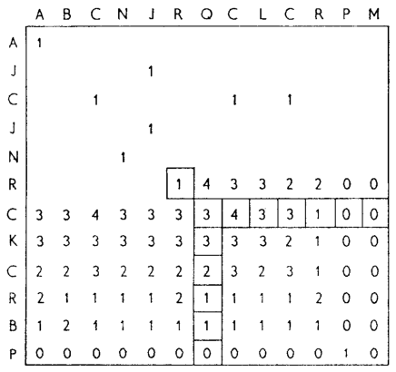
Figure 3: The cubic algorithm of Needleman and Wunsch (1970).
TODO: max instead of min formulation
This algorithm (wikipedia) defines \(S(i,j)\) as the score of the best path ending with a (mis)match in \((i,j)\). The recursion uses that before matching \(a_{i-1}\) and \(b_{j-1}\), either \(a_{i-2}\) and \(b_{j-2}\) are matched to each other, or one of them is matched to some other character:
\begin{align} S(0,0) &= S(i,0) = S(0,j) := 0\\ S(i,j) &:= \delta(a_{i{-}1}, b_{j{-}1})&& \text{cost of match}\\ &\phantom{:=} + \max\big( \max_{0\leq i’ < i} S(i’, j{-}1) + w_{i{-}i’{-}1},&&\text{cost of matching $b_{j-2}$}\\ &\phantom{:=+\max\big(} \max_{0\leq j’<j} S(i{-}1, j’)+w_{j{-}j’{-}1}\big).&&\text{cost of matching $a_{i-2}$} \end{align}
The value of \(S(n,m)\) is the score of the alignment.
Note that the original paper uses \(MAT_{ij}\) notation and goes backwards instead of forwards. The example they provide is where \(\delta(a_i, b_j)\) is \(1\) when \(a_i=b_j\), and thus computes the length of the LCS. Figure Figure 3 shows the dependencies in the evaluation of a single cell. The total runtime is \(O(nm \cdot (n+m)) = O(n^2m)\) since each cell needs \(O(n+m)\) work.
A quadratic DP Link to heading
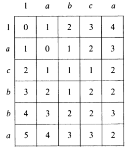
Figure 4: An example of the edit distance computation between two sequences as shown in Sellers (1974), using unit costs. 1 is a special character indicating the start.
Sellers (1974) and Wagner and Fischer (1974) both provide the following quadratic recursion for edit distance. The improvement here compared to the previous cubic algorithm comes from dropping the requirement that \(D(i,j)\) has a (mis)match between \(a_i\) and \(b_j\), and dropping the gap cost \(w_k\).
\begin{align} D(i, 0) &:= \sum_{0\leq i’ < i} \delta(a_i, -) \\ D(0, j) &:= \sum_{0\leq j’ < j} \delta(-, b_j)\\ D(i, j) &:= \min\big(D(i{-}1,j{-}1) + \delta(a_i, b_j), &&\text{(mis)match}\\ &\phantom{:=\min\big(}\, D(i{-}1,j) + \delta(a_i, -), && \text{deletion}\\ &\phantom{:=\min\big(}\, D(i,j{-}1) + \delta(-, b_j)\big). && \text{insertion}. \end{align}
This algorithm takes \(O(nm)\) time since it does constant work per DP cell.
History and naming: This algorithm is now called the Needleman-Wunsch (NW) algorithm (wikipedia). Gotoh (1982) refers to it as Needleman-Wunsch-Sellers’ algorithm, to highlight the speedup that Sellers (1974) contributed. Apparently Gotoh was not aware of the identical formulation in Wagner and Fischer (1974).
Vintsyuk (1968) is a quadratic algorithm published already before Needleman and Wunsch (1970), but in the context of speech recognition, where instead of characters there is some cost \(d(i,j)\) to match two states. It does not allow deletions, and costs are associated with a state \((i,j)\), instead of the transitions between them:
\begin{align} D(i, j) &:= \min\big(D(i{-}1,j{-}1), D(i{-}1, j)\big) + \delta(i,j). \end{align}
The quadratic recursion of Sankoff (1972) is similar to the one by Sellers (1974), but similar to Needleman and Wunsch (1970) this is a maximizing formulation. In particular they set \(\delta(a_i, b_j)=1\) when \(a_i = b_j\) and \(0\) otherwise, so that they compute the length of the LCS. This leads to the recursion
\begin{align} S(i, j) &:= \max\big(S(i{-}1,j{-}1) + \delta(a_i, b_j),\, D(i{-}1, j), D(i, j{-}1)\big). \end{align}
The wiki pages on Wagner-Fisher and Needleman-Wunsch have some more historical context.
Local alignment Link to heading
Smith and Waterman (1981) introduces local alignment (wikipedia). This is formulated as a maximization problem where matching characters give positive score \(\delta(a,b)\). The maximum includes \(0\) to allow starting a new alignment anywhere in the DP table, ‘discarding’ parts that give a negative score. The best local alignment corresponds to the larges value \(S(i,j)\) in the table.
\begin{align} S(0, 0) &:= S(i, 0) = S(0, j) := 0 \\ S(i,j) &:= \max\big(0, &&\text{start a new local alignment}\\ &\phantom{:=\max\big(} S(i-1, j-1) + \delta(a_{i{-}1}, b_{j{-}1}), &&\text{(mis)math}\\ &\phantom{:=\max\big(} \max_{0\leq i’ < i} S(i’, j) - w_{i{-}i’}, &&\text{deletion}\\ &\phantom{:=\max\big(} \max_{0\leq j’<j} S(i, j’)-w_{j{-}j’}\big).&&\text{insertion} \end{align}
This algorithm uses arbitrary gap costs \(w_k\), as first mentioned in Needleman and Wunsch (1970) and formally introduced by Waterman, Smith, and Beyer (1976). Because of this, it runs in \(O(n^2m)\).
History and naming: The quadratic algorithm for local alignment is now usually referred to as the Smith-Waterman-Gotoh (SWG) algorithm, since the ideas in Gotoh (1982) can be used to reduce the runtime from cubic by assuming affine costs, just like to how Sellers (1974) sped up Needleman and Wunsch (1970) for global alignment costs by assuming linear gap costs. Note though that Gotoh (1982) only mentions this speedup in passing, and that Smith and Waterman could have directly based their idea on the quadratic algorithm of Sellers (1974) instead.
Affine costs Link to heading
In their discussion, Smith, Waterman, and Fitch (1981) make the first mention of affine costs that I am aware of. Gotoh (1982) generalized the quadratic recursion to these affine costs \(w_k = o + k\cdot e\), to circumvent the cubic runtime needed for the arbitrary gap costs of Waterman, Smith, and Beyer (1976). He introduces two additional matrices \(P(i,j)\) and \(Q(i,j)\) that contain the minimal cost to get to \((i,j)\) where the last step is required to be an insertion/deletion respectively.
\begin{align} D(i, 0) &= P(i, 0) = I(i, 0) := 0 \\ D(0, j) &= P(0, j) = I(0, j) := 0 \\ P(i, j) &:= \min\big(D(i-1, j) + o+e, &&\text{new gap}\\ &\phantom{:= \min\big(}\ P(i-1, j) + e\big)&&\text{extend gap}\\ Q(i, j) &:= \min\big(D(i, j-1) + o+e, &&\text{new gap}\\ &\phantom{:= \min\big(}\ Q(i, j-1) + e\big)&&\text{extend gap}\\ D(i, j) &:= \min\big(D(i-1, j-1) + \delta(a_{i-1}, b_{j-1}),\, P(i, j),\, Q(i, j)\big). \end{align}
This algorithm run in \(O(nm)\) time.
Gotoh mentions that this method can be modified to also solve the local alignment of Smith and Waterman (1981) in quadratic time.
Minimizing vs. maximizing duality Link to heading
While the DP formulas for minimizing cost and maximizing score are very similar, there are some interesting conceptual differences.
When maximizing the score, this is a conceptually similar to computing the LCS: each pair of matching characters increases the score. Needleman and Wunsch (1970) gives an example of this. As we will see, these algorithms usually consider all pairs of matching characters between \(A\) and \(B\).
Algorithms that minimize the cost instead look at the problem as finding the shortest path in a graph, usually with non-negative weights and cost \(0\) for matching characters. The structure of the corresponding DP matrix turns out to be more complex, but can also be exploited for algorithms faster than \(O(nm)\).
Maximizing score is typically used for local alignment, since it needs an explicit bonus for each matches character. Most modern aligners are based on finding the shortest path, and hence minimize cost.
LCS: For the problem of LCS in particular there is a duality. When \(p\) is the length of the LCS, and \(s\) is the cost of aligning the two sequences via the LCS cost model where indels cost \(1\) and mismatches are not allowed, we have
\begin{align} 2\cdot p + s = n+m. \end{align}
Parameter correspondence: More generally for global alignment, Eizenga and Paten (2022) show that there is a direct correspondence between parameters for maximizing score and minimizing cost, under the assumption that each type of operation has a fixed cost3. In the affine scoring model, let \(\delta(a, a) = l_p\), \(\delta(a,b) = x_p\), and \(w_k = o_c + e_c \cdot k\). Then the maximal score satisfies
\begin{align} p = l_p \cdot L - x_p \cdot X - o_p \cdot O - e_c \cdot E, \end{align}
where \(L\) is the number of matches in the optimal alignment, \(X\) the number of mismatches, \(O\) the number of gaps, and \(E\) the total length of the gaps. From this, they derive an equivalent cost model for minimizing scores:
\begin{align} l_s &= 0\\ x_s &= 2l_p + 2x_p\\ o_s &= 2o_p\\ e_s &= 2e_p + l_p. \end{align}
Using that \(2L+2X+E=M+N\), this results in
\begin{align} s &= 0\cdot L + x_s \cdot X + o_s \cdot O+e_s \cdot E\\ &= (2l_p-2l_p) L+ (2l_p+2x_p) X + 2o_p O + (2e_p+l_p) E\\ &= l_p(2L+2X+E) - 2(l_p L - x_p X - o_p O - e_p E)\\ &= l_p\cdot (N+M) - 2p. \end{align}
This shows that any global alignment maximizing \(p\) at the same time minimizes \(s\) and vice versa.
Four Russians method Link to heading
Figure 5: In the four Russians method, the (ntimes m) grid is divided into blocks of size (rtimes r). For each block, differences between DP table cells along the top row (R) and left column (S) are the input, together with the corresponding substrings of (A) and (B). The output are the differences along the bottom row (R’) and right column (S’). For each possible input of a block, the corresponding output is precomputed, so that the DP table can be filled by using lookups only. Red shaded states are not visited. (CC0; source)
The so called four Russians method (wikipedia) was introduced by Arlazarov, Dinitz, Kronrod, and Faradzhev (1970), and who all worked in Moscow at the time of publication. It is a general method to speed up DP algorithm from \(n^2\) to \(n^2 / \lg n\) provided that entries are integers and all operations are ’local’.
Masek and Paterson (1980) apply this idea to pairwise alignment, resulting in the first subquadratic algorithm for edit distance. They partition the \(n\times m\) matrix in blocks of size \(r\times r\), for some \(r=\log_k n\), as shown in figure Figure 5. Consider the differences \(R_i\) and \(S_i\) between adjacent DP table cells along the top row (\(R_i\)) and left column (\(S_i\)) of the block. The core observation is that the differences \(R’_i\) and \(S’_i\) along the bottom row and right column of the block only depend on \(R_i\), \(S_i\), and the substrings \(a_i\cdots a_{i+r}\) and \(b_j\cdots b_{j+r}\). This means that for some value of \(k\), \(r=\log_k n\) is small enough so that we can precompute the values of \(R’\) and \(S’\) for all possibilities of \((R, S, a_i\cdots a_{i+r}, b_j\cdots b_{j+r})\) in \(O(n^2/r)\) time.
Note that \(k\) depends on the size of the alphabet, \(|\Sigma|\). In practice this needs to be quite small.
Using this precomputation, the DP can be sped up by doing a single \(O( r)\) lookup for each of the \(O(n^2/r^2)\) blocks, for a total runtime of \(O(n^2/\lg n)\).
Wu, Manber, and Myers (1996) present a practical implementation of the four Russians method for approximate string matching. They suggest a block size of \(1\times r\), for \(r=5\) or \(r=6\), and provide efficient ways of transitioning from one block to the next.
Nowadays, the bit-parallel technique (e.g. Myers (1999)) seems to have replaced four Russians, since it can compute up to 64 cells in a single step, while not having to wait for (comparatively) slow lookups of the precomputed data.
TODO \(O(ns)\) methods Link to heading
TODO: Diagonal transition only works for fixed indel cost (but may have variable mismatch cost)
TODO Exponential search on band Link to heading
TODO LCS: thresholds, $k$-candidates and contours Link to heading
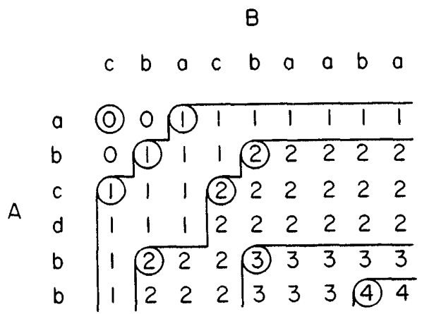
Figure 6: Contours as shown in Hirschberg (1977)
- Hunt and Szymanski (1977) [wikipedia]
- An \(O((r+n) \lg n)\) algorithm for LCS, for \(r\) ordered pairs of positions where the two sequences match, using an array of threshold values \(T_{i,k}\): the smallest \(j\) such that the prefixes of length \(i\) and \(j\) have an LCS of length \(k\). Faster than quadratic for large alphabets (e.g. lines of code).
- Hirschberg (1977)
- Defines $k$-candidates (already introduced in Hirschberg’s thesis two years before) as matches where a LCS of length \(k\) ends. Minimal (also called essential elsewhere) $k$-candidates are those for which there are no other smaller $k$-candidates. This leads to contours: the border between regions of equal $L$-value, and an \(O(pn+n\lg n)\) algorithm. His \(O(p (m-p) \lg n)\) algorithm is based on using a band of width \(m-p\) when the LCS has length at least \(p\).
TODO Diagonal transition: furthest reaching and wavefronts Link to heading
- Ukkonen Ukkonen (1983 conference, 1985 paper)
- Introduces the diagonal transition method for edit costs, using \(O(s\cdot
\min(m,n))\) time and \(O(s^2)\) space, and if only the score is needed, \(O(s)\)
space.
Concepts introduced:
\(D(i,j)\) is non-decreasing on diagonals, and has bounded increments.
Furthest reaching point: Instead of storing \(D\), we can store increments only: \(f_{kp}\) is the largest \(i\) s.t. \(D(i,j)=p\) on diagonal \(k\) (\(j-i=k\)). [TODO: they only generalize it from LCS elsewhere]
A recursion on \(f_{kp}\) for unit costs, computing wavefront \(f_{\bullet,p}\) from the previous front \(f_{\bullet, p-1}\), by first taking a maximum over insert/deletion/substitution options, and then increasing \(f\) as long as characters on the diagonal are matching.
Only \(O(s^2)\) values of \(f\) are computed, and if the alignment is not needed, only the last front \(f_{\bullet, p}\) is needed at each step.
Gap heuristic: The distance from \(d_{ij}\) to the end \(d_{nm}\) is at least \(|(i-n)-(j-m)|\cdot \Delta\) when \(\Delta\) is the cost of an indel. This allows pruning of some diagonals.
Additionally, this paper introduces an algorithm that does exponential search on the band with, leading to an \(O(ns)\) algorithm for general costs but using \(O(ns)\) space.
Mentions \(O(n+s^2)\) best case and that \(O(ns)\) is a pessimistic worst case, but no expected case.
- Myers (1986), submitted ‘85
- Independent of Ukkonen (1985), this
introduces the concept of furthest reaching point and the
recursion, but for LCS. Dijkstra’s algorithm is used to evaluate DP states in
order of increasing distance. \(O(ns)\). For random strings, they show it runs in
\(O(n+s^2)\) expected time.
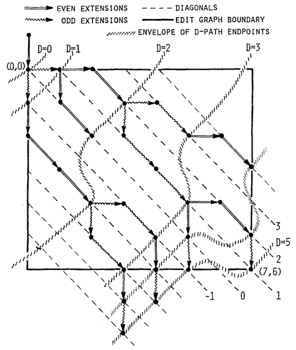
Figure 7: Furthest reaching points for LCS by Myers (1986).
Uses divide-and-conquer to achieve \(O(n)\) space; see below.
- Landau and Vishkin (1989), submitted ‘86
- Extends Ukkonen (1985)
to $k$-approximate string matching, the problem of finding all matches of a
pattern in a text with at most \(k\) errors, in
\(O(nm)\) time. They improve this to \(O(nk)\) by using a suffix tree with LCA
queries to extend matching diagonals in \(O(1)\) instead of checking one
character at a time.

Figure 8: Example of Landau and Vishkin (1989). Note that values increase along diagonals.
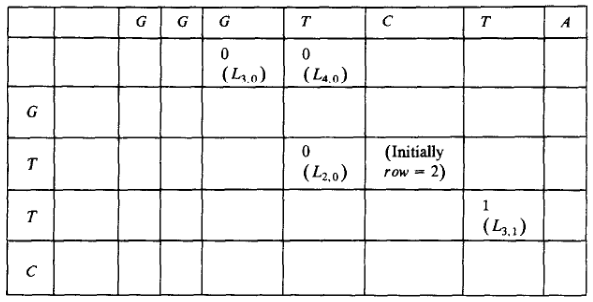
Figure 9: Furthest reaching points for the above example.
TODO Suffixtree for \(O(n+s^2)\) expected runtime Link to heading
Using less memory Link to heading
Computing the score in linear space Link to heading
Gotoh (1982) was the first to remark that if only the final alignment score is needed, and not the alignment itself, linear memory is often sufficient. Both the quadratic algorithms presented above can use this technique. Since each column \(D(i, \cdot)\) of the matrix \(D\) (and \(P\) and \(Q\)) only depends on the previous column \(D(i-1, \cdot)\) (and \(P(i-1, \cdot)\) and \(Q(i-1, \cdot)\)), it suffices to only keep those in memory while computing column \(i\).
Divide-and-conquer Link to heading
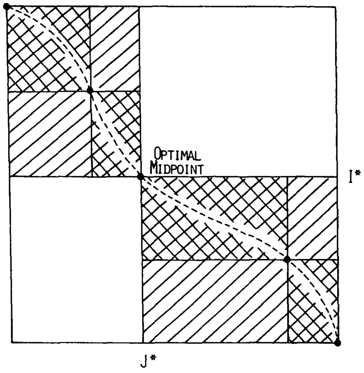
Figure 10: Divide-and-conquer as shown in Myers and Miller (1988). Unlike the text here, they choose i* to be the middle row instead of the middle column.
Hirschberg (1975) introduces a divide-and-conquer algorithm to compute the LCS of two sequences in linear space. This technique was applied multiple times to reduce the space complexity of other algorithms as well: Myers (1986) applies it to their \(O(ns)\) LCS algorithm, Myers and Miller (1988) reduces the \(O(nm)\) algorithm by Gotoh (1982) to linear memory, and biWFA [unpublished] improves WFA.
Method: Instead of computing the alignment from \((0,0)\) to \((n,m)\), we fix \(i^\star = \lfloor n/2\rfloor\) and split the problem into two halves: We compute the forward DP matrix \(D(i, j)\) for all \(i\leq i^\star\), and introduce a backward DP \(D’(i, j)\) that is computed for all \(i\geq i^\star\). Here, \(D’(i,j)\) is the minimal cost for aligning suffixes of length \(n-i\) and \(m-j\) of \(A\) and \(B\). A theorem of Hirschberg shows that there must exist a \(j^\star\) such that \(D(i^\star, j^\star) + D’(i^\star, j^\star) = D(n, m)\), and we can find \(j^\star\) as the \(j\) that minimizes \(D(i^\star, j) + D’(i^\star, j)\).
This means that the point \((i^\star, j^\star)\) is part of the optimal alignment. The two resulting subproblems of aligning \(A[0, i^\star]\) to \(B[0, j^\star]\) and \(A[i^\star, n]\) to \(B[j^\star, m]\) can now be solved recursively using the same technique, where again we find the midpoint of the alignment. This recursive process is shown in figure Figure 10. The recursion stops as soon as the alignment problem becomes trivial.
Space complexity: At each step we can use the linear-space variant described above to compute \(D(i^\star, j)\) and \(D’(i^\star, j)\) for all \(j\). Since we only do one step at a time and the alignment itself (all the pairs \((i^\star, j^\star)\)) only takes linear space as well, the overall space needed is linear.
Time complexity: This closely follows Myers and Miller (1988). The time taken in the body of each step (excluding the recursive calls) is bounded by \(C\cdot mn\) for some constant \(C\). From figure Figure 10 it can be seen that the total time spent in the two sub-problems is \(\frac 12 C\cdot mn\), as the corresponding shaded area is half the of the total area. The four sub-sub-problems again take half of that time, and a quarter of the total time, \(\frac 14 C\cdot mn\). Summing over all layers, we get a total run time bounded by
\begin{equation} C\cdot mn + \frac 12 C\cdot mn + \frac 14 C\cdot mn + \frac 18C\cdot mn + \dots \leq 2C\cdot mn = O(mn). \end{equation}
In practice, this algorithm indeed takes around twice as long to find an alignment as the non-recursive algorithm takes to find just the score.
TODO LCSk[++] algorithms Link to heading
- (Benson, Levy, and Shalom 2013) introduces LCSk: LCS where all matches come \(k\) characters at a time. Presents a quadratic NW-like algorithm.
- (Pavetić, Žužić, and Šikić 2014) introduces LCSk++, and an algorithm for it with expected time \(O(n + r \lg r)\), where \(r\) is the number of $k$-match pairs, similar to (Hunt and Szymanski 1977).
- (Deorowicz and Grabowski 2014) Overview of LCS algorithms – nothing new here.
- (Pavetić et al. 2017) more incremental improvements – not so interesting
Theoretical lower bound Link to heading
Backurs and Indyk (2018) show that Levenshtein distance can not be solved in time \(O(n^{2-\delta})\) for any \(\delta > 0\), on the condition that the Strong Exponential Time Hypothesis (SETH) is true. Note that the \(n^2/\lg n\) runtime of the four Russians method is not \(O(n^{2-\delta})\) for any \(\delta>0\), and hence does not contradict this.
They use a reduction from the Orthogonal Vectors Problem (OVP): given two sets \(A, B\subseteq \{0,1\}^d\) with \(|A|=|B|=n\), determine whether there exists \(x\in A\) and \(y\in B\) such that \(x\cdot y=\sum_{j=1}^d x_j y_j\) equals \(0\). Their reduction involved constructing a string (gadget) \(VG’_1(a)\) for each \(a\in A\) and \(VG’_2(b)\) for each \(b\in B\), such that \(EDIT(VG’_1(a), VG’_2(b))\) equals \(C_0\) if \(a\cdot b=0\) and equals \(C_1>C_0\) otherwise. Then they construct strings
\begin{align} P_1 &= VG’_1(a_1) \cdots VG’_1(a_n)\\ P_2 &= \big[VG’_2(f)\big]^{n-1} \cdot \big[VG’_2(b_1) \cdots VG’_2(b_n)\big] \cdot \big[VG’_2(f)\big]^{n-1} \end{align}
for some fixed element \(f\), and conclude that the cost of a semi-global alignment of \(P_1\) to \(P_2\) is some constant \(X\) if \(a\cdot b=0\) is not possible, and at most \(X-2\) otherwise.
If edit distance can be computed in strongly subquadratic time, then so can semi-global alignment. Using the reduction above that would imply a subquadratic solution for OVP, contradicting SETH.
TODO A note on DP (toposort) vs Dijkstra vs A* Link to heading
TODO: Who uses/introduces gap heuristic?
TODO: ukkonen'85 (first?) states the link between DP and shortest path (in edit graph)
TODO: Include Fickett 84 paper for O(ns) variant of dijkstra
TODO: https://link.springer.com/article/10.1186/1471-2105-10-S1-S10
TODO Tools Link to heading
Note: From 1990 to 2010 there is a gap without much theoretical progress on exact alignment. During this time, speedups were achieved by [TODO: citations]:
- more efficient implementations on available hardware;
- heuristic approaches such as banded alignment and $x$-drop.
There are many implementations of exact and inexact aligners. Here I will only list current competitive aligners.
[TODO: This is very incomplete for now]
- Greedy matching
- todo
- Myers bit-parallel algorithm
- todo
- SeqAN
- \(O(nm)\) NW implementation, or \(O(nm/w)\) using bit-parallel (Myers 1999) for unit cost edit distance: docs
- Parasail
- todo
- KSW2
- todo
- Edlib
- diagonal transition (Ukkonen 1985) and bit-parallel (Myers 1999)
- WFA
- exact, diagonal transition method
States the recurrence for gap-affine costs for the diagonal transition algorithm, and provides a fast implementation. It is unclear to me why it took 30+ years to merge the existing gap-affine recursion and more efficient diagonal-transition method.
- WFA2
- Extends WFA to more cost models, more alignment types, and introduces low-memory variants
- WFALM
- *L*ow *M*emory variant of WFA.
Uses a square-root decomposition to do backtracking in \(O(s^{3/2})\)
Additional speedup: The extension/greedy matching can be done using a precomputed suffixtree and LCA queries. This results in \(O(n+m+s^2)\) complexity but is not faster in practice. [TODO: original place that does this]
- biWFA [WIP, unpublished]
- Meet-in-the-middle/divide-and-conquer variant of WFA, applying the ideas in Hirschberg (1975) to WFA to reconstruct the alignment in linear space.
- lh3/lv89
- Similar to biWFA (but non-recursive) and WFALM (but with a fixed edit-distance between checkpoints, instead of dynamically storing every \(2^{i}\) th wavefront).
TODO Notes for other posts Link to heading
Semi-global alignment papers Link to heading
- (Landau and Vishkin 1989)
- (Myers 1999)
- (Chang and Lampe 1992): shows that ukkonens idea (Finding approximate patterns in strings, also ‘85) runs in \(O(nk)\) expected time for $k$-approximate string matching, when the reference is a random string.
- (Wu, Manber, and Myers 1996): Efficient four russians in combination with ‘ukkonens zone’ \(O(kn/\lg s)\) when \(O(s)\) space is available for lookup.
- Baeza-Yates Gonnet 92
- Baeza-Yates Navarro 96
- https://www.biorxiv.org/content/10.1101/133157v3
Approximate pairwise aligners Link to heading
- Block aligner
Old vs new papers Link to heading
There’s a big dichotomy between the old and the new papers:
old
- short intro
- to the point
- little context; more theory
- short about utility: Gotoh has literally 1 sentence on this: ‘can be executed on a small pc with limited memory’
- Examples: (Smith and Waterman 1981), the original four russians paper
new
- at least 1 A4 of blahblah
- needs to talk about other tools, types of data available (length and error rate of pacbio…)
- spends 3 pages on speed compared to others
References Link to heading
The paper introducing glocal alignment (Brudno et al. 2003), actually defines that as something else… ↩︎
also arbitrary gaps? ↩︎
Is it possible to extend this to arbitrary mismatch costs \(\delta(a,b)\)? Probably not since the proof relies on the LCS duality. ↩︎