There was a hackernews post recently on a new single-source shortest path algorithm (Duan et al. 2025), that takes \(O(m (\log n)^{2/3})\) time, which is less than \(O(m + n \log n)\) (the complexity of Dijkstra with Fibonacci heaps with \(O(1)\) inserts) when \(m \leq n (\log n) ^{1/3}\), or equivalently, when the average degree satisfies \(d=m/n=O((\log n) ^{1/3})\). Anyway – this got me thinking about heaps. Specifically, about how fast we can make them.
The bottom line is that there is the quickheap data structure (Navarro and Paredes 2010) and its improved version (Navarro et al. 2011), and my implementation of this (github:ragnargrootkoerkamp/quickheap) is 2 to 3\(\times\) faster than the other heaps/priority queues from crates.io that I tested.
As for the title: there are many papers on I/O efficient and cache-oblivious heaps and priority queues (Brodal 2013), but I am not able to find a modern implementation of any one of them – somehow they don’t seem used at all in practice. On the other hand, there is the radix heap (Ahuja et al. 1990) that is faster at times, but it can only be used in cases where the extracted keys increase with time.
Jump straight to Implementation or Results.
1 Background Link to heading
Priority queue Link to heading
As a quick recap, for the purposes of this post, a priority queue (wikipedia) is a data structure that supports the following two operations:
- Push (insert)
- Add a value \(x\) to the data structure.
- Pop (extract min)
- Remove and return the smallest value \(x\) in the data structure.
Other possible operations include find min (peek), delete, and decrement key, but we will not consider these.
Note: most literature seems to present the min-queue as above, but Wikipedia and implementations often use a max-queue, where a pop returns the maximum element instead.
Binary heap Link to heading
The binary heap (wikipedia) works by using the Eytzinger layout, also known as simply the heap layout. This represents \(n\) values as a binary tree that is stored layer by layer. If we put the root at index 1, the children of node \(i\) are at \(2i\) and \(2i+1\). The heap invariant, which makes the tree into a heap (wikipedia), is that each value is at most the value of its two children, which implies that the root is the smallest value.
Push is implemented by first appending the new value to the array, which adds it as the next node in the bottom layer of the tree (or possibly creating a new layer). Then, we ensure the invariant is preserved by swapping the new element with its parent as long as its larger.
Pop is implemented by first extracting the root, and replacing it with the last element of the queue. Then, we again ensure the invariant is preserved by sifting down: we swap the root with the smaller of its two children as long as needed.
We can see that in the worst case, both these operations take \(\lg n = \log_2(n)\) steps.
D-ary heaps Link to heading
D-ary heaps (wikipedia) generalize binary heaps so that each node has up to \(d\) children. Their main benefit is that they have better cache locality, and require fewer levels of traversing the tree. The drawback is that sifting down requires finding the minimum of \(d\) elements rather than just 2, but this is anyway fast using some SIMD instructions.
Other heaps Link to heading
Other heaps are the radix heap (wikipedia, nice blog explanation) (Ahuja et al. 1990), which implements a monotone priority queue where the priority of the popped elements may only increase. This is for example the case when running Dijkstra’s algorithm on a graph with non-negative edge weights.
The sequence heap (Sanders 2000) and funnel heap (Brodal and Fagerberg 2002) are two similar I/O efficient / cache-oblivious data structures. (But, according to Brodal (2013), they serve slightly different purposes.) They build on the idea of binary mergers: given two input buffers containing sorted data, they merge those into a sorted output buffer as needed. These “gadgets” are used to build $k$-way mergers, and a chain of these is made for exponentially increasing \(k\).
The cascade heap (Babenko, Kolesnichenko, and Smirnov 2017) has \(O(1)\) inserts, and \(O(\log^* n + \log k)\) pop for the \(k\)’th popped element. Thus, this avoids the overhead of doing too much up-front work. The logarithmic funnel (Loeffeld 2023) takes a similar approach of building high dimensional trees.
A more broad survey is given by Brodal (2013), which surprisingly does not mention the quickheap described below.
2 Literature on Quickheaps Link to heading
Sorting algorithms go back a long way. One way to sort a list is to put all elements in a heap and then extract them one by one, called heapsort (Williams 1964).
Another method is quicksort, which works as follows: first, choose a random element of the array as pivot. Then compare all elements to this pivot, and move the smaller ones to the front of the array, and the larger ones to the back of the array. Then recurse on the two halves. This runs in \(O(n\log n)\) time, since the number of levels in the recursion is expected to be \(O(\log n)\).
Optimal incremental sorting Link to heading
A related problem is to only sort the smallest \(k\leq n\) elements, which can be done in \(O(n + k \log k)\). Heapsort does this, but incurs an up-front cost of \(O(n \log n)\). Paredes and Navarro (2006) give an incremental \(O(n+k\log k)\) method that returns the smallest elements one by one in sorted order. Their method, IncrementalQuickSelect (IQS) builds on the ideas of quicksort:
- Choose a random pivot and partition the array.
- Push the position of the pivot to a stack.
- Recurse on the left part with smaller values until only a single element is left. This is the minimum.
- Pop that element, go up the stack, and recurse on the elements between this pivot and the next as needed.
- Repeat until the array is empty.
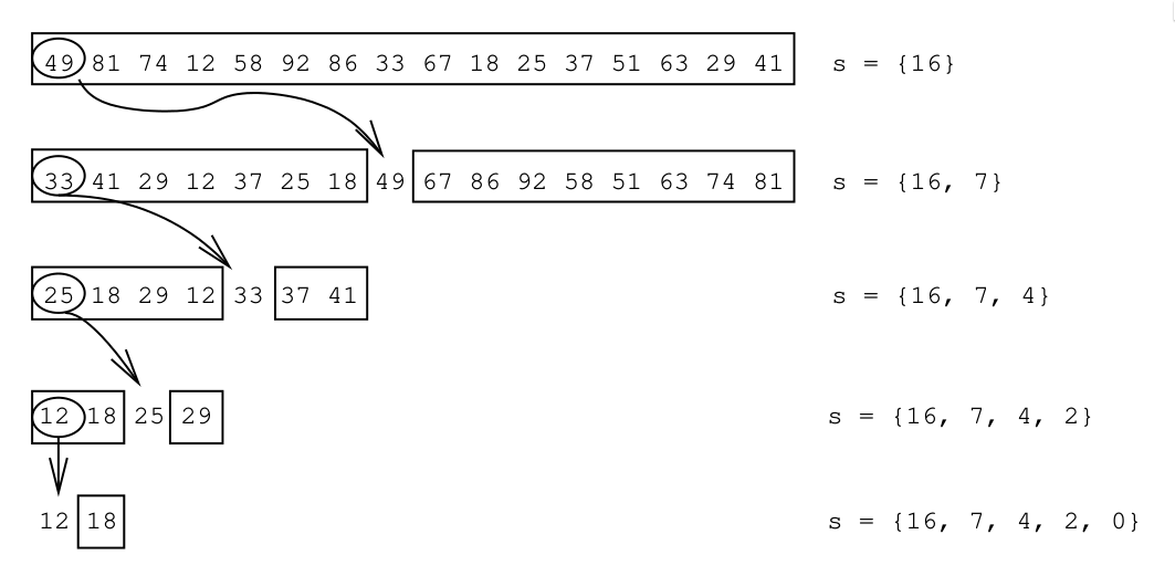
Figure 1: Example from Paredes and Navarro (2006) of the IQS method: a random (here: first) element is chosen as pivot to partition the array. This is repeated until only a single element is left, and the positions of all pivots are stored on a stack.
On random input, IQS takes average time \(O(n + k \log k)\).
Quickheap Link to heading
The conclusions of the 2006 paper above already mention that this same idea can be used to build a heap. This is presented in detail in Navarro and Paredes (2010).
Compared to the incremental sorting method above, the one additional operation it needs to support is pushing new elements.
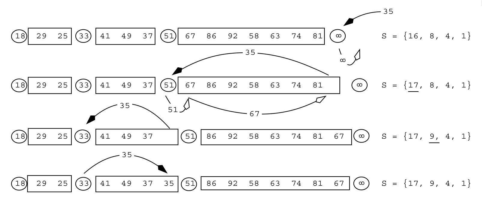
Figure 2: Example from Navarro and Paredes (2010) of inserting an element (35) into the quickheap.
Like with binary heaps, we first push the new element to the back of the array, and then sift it (down, in this case) to its right location: as long as the new element is less than the preceding pivot, that pivot (eg 51 above) is shifted one position to the right to make space for the new element, and the new element is inserted on its left.
Since the tree is expected to have \(O(\log n)\) many levels on random input, this takes \(O(\log n)\) steps, as for binary heaps. Additionally, it is shown that the I/O cost of push and pop is \(O((1/B) \log (m/M))\), where \(B\) is the block size and \(M\) is the total available memory, which is close to optimal. Thus, quickheaps make efficient use of the memory bandwidth.
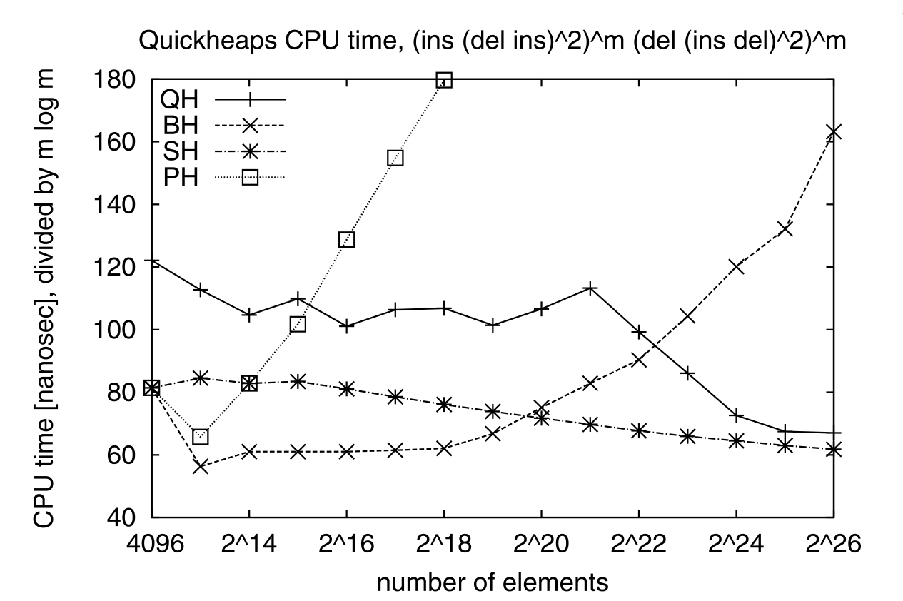
Figure 3: On a sequence of m times (ins, (del, ins)^2) followed by m times (del, (ins, del)^2), quickheap (QH) is faster than the binary heap (BH) and pairing heap (PH), but slightly slower than the sequence heap (SH), which are optimized for cases where all elements are extracted. Note that the y-axis reports the time divided by m lg(m).
Quickheaps are also shown to have much lower I/O cost than radix heaps.
A drawback of quickheaps is that the analysis only works for randomized operations.
Randomized quickheaps Link to heading
When the keys being inserted into quickheap are mostly decreasing, this causes the number of layers/pivot to grow over time. This results in worst-case linear time inserts, since elements have to sift down linearly many layers.
Randomized quickheaps (RQH) (Navarro et al. 2011) solve this: every time an element is inserted and moves down one layer, the entire subtree starting in that layer is flattened with probability \(1/s\) when it has \(s\) elements. That is, all pivots in the subtree are dropped, and the next pop operation will pick a new random pivot. This way, each subtree is re-randomized roughly once each time it doubles in size.
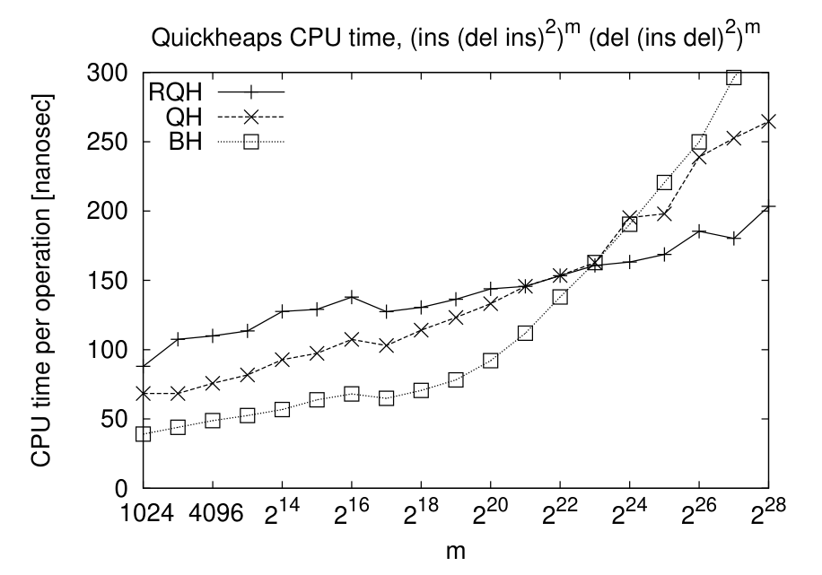
Figure 4: On a sequence of m times (ins, (del, ins)^2) followed by m times (del, (ins, del)^2), the random quickheap (RQH) is faster than both the binary heap (BH) and quickheap (QH) for sufficiently large inputs.
The paper by Regla and Paredes (2015) takes a more practical approach to optimal worst-case behaviour. One could use the median-of-medians algorithm to select a pivot in the 30%-70% interval in linear time, but this is slow in practice. Instead, they first try a random pivot, and only fall back to median-of-medians in case this random pivot is not in the 30%-70% interval.
3 Bucket-based implementation Link to heading
Data structure Link to heading
The original quickheap papers store everything in a flat array, without additional memory. In my implementation (github), I instead use a single bucket (vector) per layer. This simplifies the partition steps, since they do not have to be in-place, but comes at the cost of somewhat higher memory usage. Additionally, I store a flat list of the pivot values for all layers, rather than their positions. Lastly, I stop the recursion when layers have size at most 16. Then, this list is simply scanned to extract the smallest element.

Figure 5: A schematic overview of the quickheap: elements are stored in layers. Deeper layers have smaller values, with each layer being at most its pivit. The bottom layer has at most 16 (here: 4) elements. Popping is done by scanning the bottom layer, and pushing is done by comparing the new value to all pilots and appending to the correct layer. To split a layer, a random pivot is selected as the median of 3 and smaller elements are pushed to the next layer, while larger elements stay. Values equal to the pivot are pushed down if they are on its left.
| |
QuickHeap data structure.The active/last layer is stored separately, so that we can reuse buffers instead of deallocating them.
Push Link to heading
Push is implemented by simply comparing the new element against all the pivots, and then inserting it into the right layer.
Code for pushing a new value.
| |
To enable maximum efficiency of SIMD comparisons, in practice we do this:
| |
This has complexity \(O((\log n)/L)\) when using \(L\) SIMD lanes, which in practice
is fast, especially when \(L=8\) for u32 values.
One option for some speedup could be to turn this into a 2-level B-tree, with a
root node that divides the levels into \(L+1\) chunks.
Pop Link to heading
Pop is more tricky. We split the current (bottom) layer as long as it has more than 16 elements. Then, we find the position of the minimum and remove it by swapping it with the last element in the layer. Lastly, we decrease the active layer if we exhausted it.
Code for popping the smallest value.
| |
Partition Link to heading
This leaves only the partitioning of the layers. Of note are the fact that I use the median of 3 candidate pivots, and that the partitioning is based on AVX2 SIMD instructions inspired by Daniel Lemire’s blog (see github for the detailed code).
Code for partitioning the bottom layer.
| |
< pivot to one and values >= pivot to the other.4 Results Link to heading
Libraries Link to heading
I benchmarked against a few heap and priority queue crates. I did not find any implementation of (randomized) quickheap either online or in the papers1, but there are some d-ary heaps:
std::collections::BinaryHeap: a plain binary max-heap. Used withReverse<u32>to make it a min-heap.orx_priority_queue::DaryHeap<(), u32, D>: a d-ary heap, tested for D in 1,2,4,8.dary_heap::DaryHeap<u32, D>: another d-ary heap, tested for D in 1,2,4,8.
Excluded implementations.
std::collections::BTreeSet: does not natively support duplicate elements, and also ~2x slower than other methods.indexset::BTreeSet: idem.fibonacci_heap::FibonacciHeap: a Fibonacci heap, but 10x slower than everything else.pheap::PairingHeap: a pairing heap, but slower than other heaps.
We do compare against a radix heap, which is specialized for cases where the popped keys increase with time.
Datasets Link to heading
I test on a few types of data. First off, we test keys with types:
u32u64
For each type, we construct a number of test cases. Each has the structure \[ F_k(n) := (\mathsf{push}\circ(\mathsf{pop}\circ\mathsf{push})^k)^n \circ(\mathsf{pop}\circ(\mathsf{push}\circ\mathsf{pop})^k)^n. \]
- Heapsort: \(F_0(n)\): \(n\) random pushes, followed by \(n\) pops. I.e. a heapsort.
- Random: \(F_4(n)\) with random pushes. This simulates a heap that slowly grows and then slowly shrinks.
- Linear: \(F_4(n)\), where the $i$th push pushes value \(i\).
- Increasing: \(F_4(n)\), but pushes increase by a random amount:
- for
u32: the last popped value plus a random value up to 1000. - for
u64: the last popped value plus a random value up to \(2^{32}\).
- for
Results Link to heading

Figure 6: (Click to enlarge.) Log-log plots of the average time per push-pop pair. Top row: u32 values, bottom row: u64 values. Left to right corresponds to the four datasets listed above: heapsort, random, linear, and increasing. The shown time is the total time divided by (2k+1), and thus is the average time for an element to be pushed and popped again. Experiments are stopped once they take >100 ns. Memory usage is 4 or 8 times more than (n), and ranges from 8 KiB to 128 MiB for u32 and double that for u64.
Some observations:
- The binary heap (blue) and d-ary heaps (orange, green) have similar
performance for
u32andu64. - The 4-ary heap (green) in
orx_priority_queueis consistently slightly faster than the default binary heap. - The 8-ary heap in
dary_heapis usually much slower, but slightly faster for large \(n\).- (Other d-ary heap variants are only rarely better than both of these two.)
- The quickheap (red) is the fastest for both heapsort and the interleaved
variant with random pushes.
- For heapsort, it’s up to 2x faster for
u32for large \(n\), because most time is spent partitioning lists, and this is 2x faster for the smaller data type. - For random interleaved pushes, this difference is nearly gone. Most likely this is because roughly 75% of pushed elements will directly be popped again. In fact, the performance is nearly independent of \(n\) here!
- Exact linear pushes are probably the worst for quickheap, as these always get pushed to the top layer and then need to sift down through the maximum possible number of layers.
- For heapsort, it’s up to 2x faster for
- The radix heap (purple) has constant performance for heapsort, since its
\(O(n\log C)\) term only depends on the number of bits in the input values,
which is 32 or 64. This is also the worst possible input for radix sort.
- Random pushes interleaved with pops are not supported, since the minimum value in the heap may only increase.
- Radix sort is the fastest for linear input, likely because of its cache locality.
- For
u32input that increases by 0 to 1000 on each push, radix sort gets faster as \(n\) increases, probably because there are very many duplicate elements. - For
u64input that increases by 0 to \(2^{32}\) on each push, radix sort is not as good, because now \(\log C=\log2^{32}\) is quite large (compared to \(\log 1000\) before). As in the heapsort case, the performance is constant though, because \(\log C\) is constant.
5 Conclusion Link to heading
Overall, the radix heap is probably a good choice in cases where it can be used, specifically for small integer input. Otherwise, the quickheap is significantly faster than binary/d-ary heaps, especially as \(n\) grows. This is primarily because of its better cache efficiency and corresponding I/O complexity: Binary/d-ary heaps must access \(O(\log n)\) memory locations and have a cache miss (of cost \(\sqrt {2^i}\), see this blog on The Myth of RAM) at each layer \(i\), whereas the quickheap pushes to one of \(O(\log n)\) known (cached) locations, pops from a single location, and has memory-efficient partitioning as well.
6 Still TODO Link to heading
- Implement the ideas from the randomized quickheap Navarro et al. (2011) to
prevent the worst-case quadratic growth.
- Or other theoretical rebalancing ideas?
- Run experiments on some more realistic datasets:
- Dijkstra with the radix heap vs quickheap
- Prim’s minimal spanning tree algorithm (wikipedia) is a case where the radix heap will not work, and might be a good case to show the improvement of the quickheap over d-ary heaps.
- Are there non-graph applications of heaps? Things like an ’event queue’ come to mind: when processing a sorted list of intervals, we push the end of the interval after processing the start. But again a radix heap (or even a bucket heap) is probably better here, unless the timestamps are very high precision.
- https://github.com/raphinesse/s3q/issues/1#issuecomment-3194478295
- https://github.com/raphinesse/s3q/releases/tag/thesis-tuned-spq
- Further extensions:
- Multithreading? Handing out batches of elements at a time and slightly losing optimality guarantees.
Possible publications:
- ESA B, deadline April 21
- PPoPP, deadline autumn 2026
- SEA deadline Jan 2027
7 Literature Link to heading
- introduces the binomial queue (not ‘binomial heap’ apparently, because the structure is a forest of heaps?)
- binomial heap has time \(O(I + D \lg I)\) for \(I\) insertions and \(D\) deletions
- amortized \(O(1)\) insert
- amortized \(O(\lg n)\) deletemin
- (same perf as binomial heap)
- but also has constant time decrease-key
- IO-model: best = 1/B log (N/B) IO/s. I think we reach that too.
- without decrease-key: 1/B log(N/B) / log(M/B) is possible, lower bound for
comparison-based sorting
- we don’t care about decrease-key
- 1/B log B / (log log N) lower bound when decrease-key is supported
- O(1/B log N/B / log log N) possible
- N: max size
- Fibonacci heap is optimal for comparison-only model.
- Complexity O(a + b lg n), a = inserts, b=deletes
- integers: each op in log log (N), or expected amortized sqrt(log log N).
- IO model:
- M: small memory size (in #words)
- big memory of blocks of B words
- each word has w=lg(N) bits
- comparison based sorting in at least n lg n
- so priority queue of size n has ‘update’=push+pop complexity at least lg n
- mostly theoretical
- push-pop on array of size \(m\) is at least \(\lg m\).
- binomial heap is optimal is # comparisons
(Sanders 2000):
- Peter’s 2000 paper
- merge buffers and such
- more like quicksort, with ‘global’ pivots and overflow buffers
- probably SOTA implementation; benchmark with FFI
- queue version of (Sanders and Winkel 2004)?
- some benchmark notes here: https://github.com/raphinesse/s3q/issues/1
- not exactly sure what’s new here on quick scan
- mostly for sorting; ~ \(n \lg n + 0.35 n\) comparisons
- bounded by \(1.5n\lg n - 0.4n\)
https://hjemmesider.diku.dk/~jyrki/Presentation/Dagstuhl-2013-09-23.pdf
- Nice compact slide overview
- lower bound: Omega(1) insert, lg(N)-(1) comparisons per extract-min
- metrics:
- element moves
- instructions
- branch mispredictions
- cache misses
- adding decrease operations makes a separate class
- ACM opinion piece on binary heap vs B-heap
- B-heap: branching factor 2, but eytzinger-like layout for better memory locality
(Larkin, Sen, and Tarjan 2013)
- Cites some ~1995 papers as most recent general benchmarks. By now, 2014 is also kinda old in fact.
- seems like a nice/good paper in general
- empirical study by Tarjan and others
The theory community has proposed several new heap variants in the recent past which have remained largely untested experimentally. We take the field back to the drawing board, with straightforward implementations of both classic and novel structures using only standard, well-known optimizations.
- random insert + pop is degenerate
- L1 cache misses predict runtime
- either insert or delete must be at least \(\Omega(\lg n)\) (and cites Knuth for this)
In practice, the worst-case of log n is often not encountered or can be treated as a constant, and for this reason simpler struc- tures with logarithmic bounds have traditionally been favored over more complicated, constant-time alterna- tives.
- measures branch misses and cache misses
- no algorithm engineering
- Fibonacci heaps sometimes outperform d-ary heaps?!
Even a well-engineered implementation like Sanders’ sequence heap [29] can be bested by our un- tuned implementations if the workload favors a different method.
- workloads:
- heapsort
- bad: random u32 inserts
- key-decrease to random between cur and min, or to min
- n inserts, cn push-pop, c in {1,32,1024}
- Dijkstra
- Nagamochi-Ibaraki min-cut
- structured and random graphs
- ’trace files’ that first record the operations in a graph, and then execute these stand-alone
- only report results on largest problem size
- pairing heaps: O(log k) pop if minimum was inserted k heap operations ago
- [28] (1997) cited for min+rand(0, C) workload
- implicit heaps are bad when decrease-key gives a new min
- small heap sizes: implicit best
- large heap sizes: amartized structures like pairing heap
- comparison to sequence heap:
- seq heap 2x faster than implicit 4-ary tree on heapsort
- seq heap 4x faster than pairing heap on random indel (c=32)
- seq heap 1.3x slower than pairing on random indel (c=1024)
- seq heap 1.2x slower than simple-2 on one network simulation instance
- => my conclusion: sequence heap is pretty good! And we should include it.
- forest of heaps
- is a treap, somehow
- theoretical only
(Costa, Castro, and de Freitas 2025)
Dial’s algorithm: Bucket queue when edge weights are bounded
TODO: Cite bucket queue paper?
There is also multi-level bucket queue, with ‘super-buckets’ of \(\sqrt C\) buckets.
or generalized to \(k\) levels
- at that point just use a radix heap
hot-queue: multi-level bucket queue, with a small heap as the first layer/bucket.
radix-heap with fibonacci heap
anyway: just cite this for info on monotone queues. We are comparison-based and non-monotone
(Benacer, Boyer, and Savaria 2018)
- title says SIMD, but really it’s FPGA
- Parallel
- parallel; buckets; weak paper
- new good algorithm for PQ with decrease-key
- analyses slim and smooth heaps
- specifically focuses on the case of decreasing keys
- analyse what happens if we don’t have the decrease-key operation
- basically: for Dijkstra, store only nodeIDs and compare distances by looking them up on-the-fly in the distance vector.
- extractmin gives an item with current key value less than original value of all other items.
- the arxiv version of the paper was withdrawn
- Nice recent paper
- TODO: Useful overview of external memory setting
- We can charge deletions to insertions, so they can even have amortized cost 0!
- IO-optimal structures exist already
- This paper: O(1/B) inserts, ie moving the cost to the deletions
- constant-time decrease-min is not possible in IO model
- Small <=M buffer of smallest elements less than a pivot.
- Fig 1 is nice!
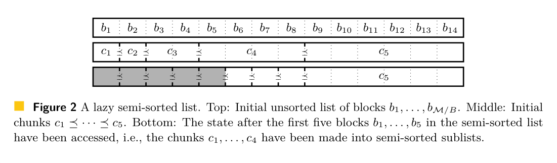
- semi-sorted list: List of sequences, such that \(X\preceq Y\) ie \(x\leq y\) for all \(x\in X, y\in Y\).
- NOTE: Figure 2 looks a lot like what we do!
The presented data structure is inherently cache-aware. This raises a natural question: does there exist a cache-oblivious priority queue that achieves the same amortized bounds on comparisons and I/Os?
- Also, currently highly amortized. Are worst-case guarantees possible?
- array-based implementation of weak heap, after introduction in (Peterson, of Technology. School of Information, and Science 1987)
- less than \(n \lg n + 0.1n\) comparisons for a heap sort
- expected around \((n-0.5)\lg n - 0.4 n\)
- lower bound for sorting is \(n\lg n - n \lg e = n\lg n - 1.44 n\)
No exact average case results exist for any of the Heapsort variants because the intermediate heaps formed during the execution of the algorithms quickly become nonrandom and it is not clear how to analyze this phenomenon.
- weak heap: root has no left subtree; nodes with <2 children are in the bottom 2 layers; heap property only holds for right subtree. The left subtree can have smaller values.
(Edelkamp, Elmasry, and Katajainen 2012)
insert in O(1) amortized time. The main idea is to temporarily store the inserted elements in a buffer, and, once the buffer is full, to move its elements to the heap using an efficient bulk-insertion procedure
- close to optimal number of comparisons, but not the fastest
(Edelkamp, Elmasry, and Katajainen 2013)
- fewer branch misses
- O(1) amortized insert via a buffer
- two buffers give wrost-case insert
- weak queue has faster delete-min than binary-heap
- cache-oblivious IO-model priority queue
- binary mergers are IO-efficient
- TODO
- See also email contact with author
- Introduces the bucket heap for BFS and shortest paths
- cache-oblivious
(Chowdhury and Ramachandran 2018)
- long paper :")
- Again familiar exponential-growth structure, but this time with 2 stack:
- one with elements
- and one with updates
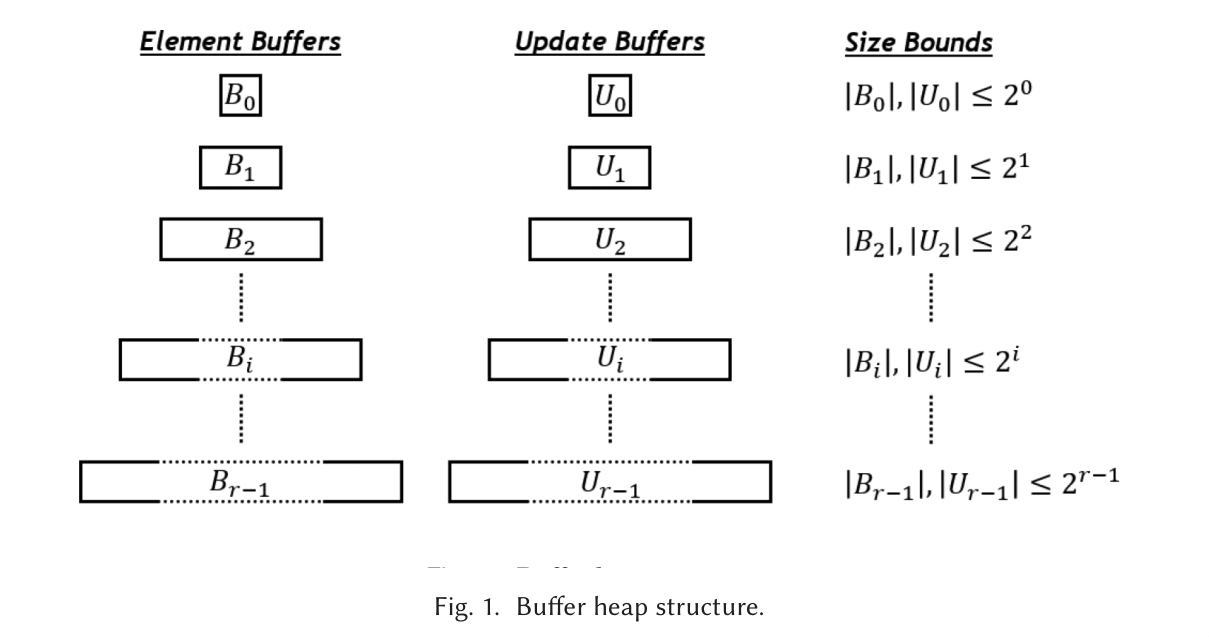
- cache-oblivious
- amortized \(O(1/B \lg (N/M))\) operations
- ensure invariants in figure are maintained. If an element or update buffer becomes to large, apply updates, and move what remains into the layer below
- redistribute: move largest key from buffer into the empty before in front. Repeat until buffer 0 is filled.
- unclear how it finds pivots / how it extracts exactly the right number of elements from each buffer
- Very similar:?!
- Nice concise previous-work
- \(O(\lg n)\) extract-min, \(O(\lg \lg n)\) insert and decrease-key
- This sounds a lot like our \(O(\lg \lg n)\) for binary-searching \(\lg n\) layers, in the case where we do rebalancing.
Not exactly sure what this means:
[QuickHeaps] Being designed for the much harder problem of keeping an entire binary search tree in shape, the resulting concatenation rules for quickheaps are complicated.
Quickheap has favorable performance in external memory model
QuickHeap excludes pointers/DecreaseKey
[One does get the feeling that this quickheap paragraph was added in hindsight?]
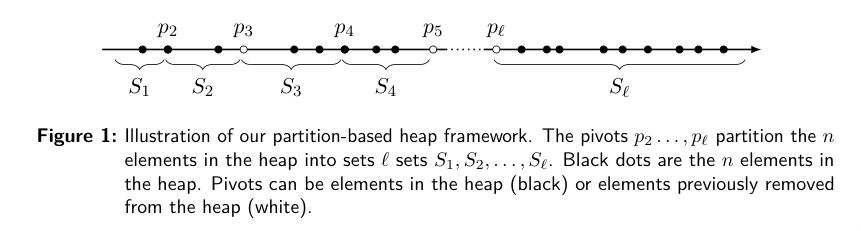
Keys are partitioned into sets \(S_1, \dots, S_\ell\) such that \(S_i \preceq S_j\) for \(i<j\). Each set is a doubly-linked-list, with stable pointers
pivots may not be present in the heap anymore
\(\lg n\) pivots
binary search in \(\lg \lg n\) time over the list of pivots for insert
Tricky part: ensuring \(\lg n\) layers
Lazy partition heaps: the sets may become arbitrarily large
Sets may not be too much larger than all preceding sets though.
Multiple variants to maintain \(\ell \leq \lg n\) invariant.
- Fibonacci variant: each layer is at most \(F_i\) large or so, so that merging up is natural. Lower bound on size of non-empty sets
pivot-forgetting rule: If the two sets separated by a pivot together are smaller than the number of elements smaller than these two sets, then merge them.
The number of layers is at most \(\ell \leq 2\lg n + 1\)
\(s(S_i)\): number of elements before \(S_i\).
potential: \(\beta \cdot (\sum_i |S_i| - s(S_i))\).
Section 3: set must be larger than the number of smaller elements
Section 4: Some complicated rules around Fibonacci numbers. I don’t get the point.
- At most 8 consecutive empty. No 2 consecutive non-empty layers.
Section 5 version: Sets are at most \(3\cdot 2^i\). Any number can be empty.
- Too large layer is pushed up, either by merging with the next larger layer or shifting both up.
- Pulling layers works by shifting down if small enough, and a select/pivot otherwise.
Using fusion trees, binary search over \(\lg n\) pivots can be done in constant time! (We sorta get the same with a \(\lg_W \lg n\) B-tree?)

- Appendix has a proof-of-concept implementation
Using our rule as the concatenation rule in quickheaps promises to yield a highly practical and robust priority queue implementation, combining the best of previously known quickheaps variants. A detailed empirical evaluation is planned for future work.
General remarks Link to heading
- There’s also a bunch of work on multi-threaded/concurrent queues, which we ignore but maybe cite a few anyway.
- Most papers are only theoretical, or focus on the number of comparisons, rather than the total running time
- Future work: types >64 bits, eg (key, value)
- I’m pretty sure we can modify our thing to be IO-optimal as well if we have a small insertion buffer.
- Not sure if we can get \(O(1)\) insertions though.
References Link to heading
There is https://github.com/emmt/QuickHeaps.jl, but it seems to just be a “quick” binary heap. ↩︎