Here, we’ll discuss some possible improvements to the SimdQuickHeap (Breitling, Groot Koerkamp, and Williams 2026) (previous post, paper PDF). Most of these came up last week during ESA, after William Kuszmaul gave a keynote on history independent data structures (specifically, layered list labelling (Bender et al. 2024)) and Marvin Williams presented our work.
I think the discussions were started by Dennis Kobert, student at KIT. They then quickly expanded to include others from KIT (Nikolai Maas, Marvin Williams, Stefan Walzer, Patrick Steil) as well as Sebastian Wild.
All together, a few ideas came up:
- A history independent quickheap (or heaps in general)
- Adding
decreaseKeysupport to the quickheap - SIMDfying the radix heap.
1 A history independent quickheap Link to heading
1.1 History independent data structures Link to heading
A dynamic data structure is history independent when the in-memory representation of, say, the set of elements is completely independent of the history of the data structure, e.g., which elements have inserted and deleted to/from it in the past.
History independence is nice for a few reasons. First, it gives the user privacy guarantees that sharing the data structure does not reveal any historical information. Second, history independence turns out to be a good way to design efficient data structures: it is impossible for the user to get the data structure in a “bad state” e.g. by repeatedly inserting and removing elements. Specifically for many hashmap implementations, such behaviour can lead to inserting many tombstones to indicate deleted elements, and these deteriorate the performance of queries.
We consider history independence for deterministic and randomized data structures. For deterministic data structures, the situation is pretty straightforward: if every represented state \(S\) has exactly one representation anyway, the data structure is trivially history independent. If deletions are allowed, it may be the case that repeatedly inserting and removing a specific element is expensive though, for example because the number of elements crosses the threshold where the data structure resizes. But in expectation over an internal random seed, or amortized over all operations, the expected cost of each operation is ideally small.
On the other hand, we could aim for a solution where the representation is a uniform random sample from some set of possible representations. This way, we are not forced to ’toggle between two states’ on repetitive insertions and deletions, and we can instead average out this cost over the internal state.
1.2 History independent list labeling Link to heading
List labeling is roughly the following problem: we have a set of \(m\) slots and maintain a dynamic set \(S\) of \(|S|=n\leq m\) elements. We can insert to \(S\), delete from \(S\), and get the current slot of an element, with the guarantee that all current elements have a different slot. (But the slot assigned to an element need not be stable.)
Typical solutions maintain the set in sorted order with empty slots in between elements to allow for future insertions.
The main idea behind the history independent algorithm of Bender, Conway, Farach-Colton, Komlós, and Kuszmaul (2024) is to assign each element a pseudo-random weight (by hashing it) and then a treap-like structure where we partition the elements into a left and right half based on the element with the smallest weight. A difference, though, is that here a somewhat balanced partition is needed, and so the split is on the smallest-priority element among the middle \(n / \lg n\) elements.
Anyway, all that we need from this is the concept of assigning pseudo-random priorities to elements and letting those decide the (then deterministic) layout of the data structure.
1.3 History independent quickheap Link to heading
At this point, Dennis Kobert had the idea to apply a similar technique to the SimdQuickHeap (just quickheap from now).
By default, we partition the elements by a median-of-3 random element, but this has two drawbacks: it’s not history independent, and the data structure can end up in a bad state where the number of layers is not \(O(\lg n)\) anymore.
Instead, we can partition each layer not by a random pivot key, but by the specific key that has the smallest pseudo-random weight (let’s call this the weight again, rather than overloading priority). This way, our data structure corresponds to the left spine of a treap. Furthermore, the layout of the data structure is fully deterministic once the seed of the hash function is chosen. On inserting a key, we find it’s bucket. Then, we compute it’s weight and if it has smaller weight than any of its parent pivots, the largest such corresponding subtree is rebuilt.
Thus, this requires that we store the weight of each pivot, and store or recompute the weight of each key during partitioning.
1.4 Duplicate elements and randomized weights Link to heading
A problem with the model above is that if we have many equal keys, they all get the same weight, which could lead to very skew distributions (for example, if 90% of the keys are equal).
As an alternative, we can choose a uniform random weight for each inserted key, rather than letting it depend on the key itself, so that identical keys have distinct weights. This makes the data structure non-deterministic: the representation of the heap is now uniform random over the set of all possible weight assignments to keys.
Initially, this requires us to store the weight of each key, so that we can re-use it once a bucket is partitioned. But it turns out this is not necessary: we can simply generate new randomness once a bucket is partitioned, as long as we generate random numbers that in the range between the weights of the two enclosing pivots.
On inserting an element, we generate its random weight, find its bucket, and rebuild all subtrees above it for which the new element has a smaller weight than the current pivot.
1.5 Stronger quickheaps Link to heading
The final realization is that in fact, we do not need to store/compute the random weight of all elements at all. Instead, we can simply take a random element to partition a bucket. To insert an element, we can directly compute the probability that its weight is less than the weight of any of the pivots above it as \(1/k\) for a subtree containing the new element that currently has \(k\) elements. Thus, on every insertion, we rebuild the entire tree with probability \(1/k_0 = 1/n\), the left subtree with probability \(1/k_1\), and so on.
But this is exactly the algorithm introduced in “Stronger Quickheaps” by Navarro, Paredes, Poblete, and Sanders (2011), under the name Randomized QuickHeap!
So, conclusion of this line of thinking: we wanted to develop history independent quickheaps (to me, mostly to speed up the data structure), and via many steps, we arrived back at the original 2012 solution :)
1.6 Order of elements Link to heading
So far, I have only considered the shape of the tree for the purposes of “the state of the data structure”, but we should also consider the order in which elements are stored in each bucket. In particular, inserting an element currently always pushes the element to the back of a bucket, but this clearly leaks information. To make the data structure fully history independent, we must keep every bucket randomly shuffled at all times. One way to do this, we think, is to choose a random index for the new element and move it there, and then taking the previous element in that location and appending it to the back of the bucket. This is similar to the Fisher-Yates shuffle algorithm.
2 QuickHeap with decreaseKey
Link to heading
Another, independent, idea is to add support for decreaseKey operations, as
these are beneficial when running e.g. Dijkstra’s algorithm in dense graphs,
where each node could be pushed as much as 10 times and it’s preferable to not
blow up the memory usage by 10x.
2.1 Some theoretical bounds Link to heading
In general, the I/O-complexity of a comparison-based priority queue is lower-bounded by \(\Omega(\frac 1B \log_{M/B} n)\) amortized I/Os per operation, which is also the minimal cost per element when sorting \(n\) items using comparisons. An $M/B$-ary variant of the binary heap with buffers of \(M\) elements in each node reaches this lower bound (Eenberg, Larsen, and Yu 2017; Sanders 2000). When decrease-key must be supported, this increases to \(\Omega(\frac 1B \log B / \log\log n)\) (Eenberg, Larsen, and Yu 2017) as a cell-probe lower bound, but note that this reduces to \(\Omega(\frac 1B)\) for \(n\gg B\). In the pointer model, a lower bound is \(\Omega(\log\log n/\log\log\log n)\) time (Iacono and Özkan 2014).
2.2 The buffer heap Link to heading
The fastest algorithm (I think; but it’s from 2018) achieves \(O(\frac 1B \log \frac nB / \log \log n)\) amortized I/Os per operation instead (Jiang and Larsen 2018).
The cache-oblivious buffer heap (Chowdhury and Ramachandran 2018) supports decrease-key in \(O(\frac 1B \log_2 \frac nM)\) I/Os and appears to be practical. Note that this is the same I/O complexity as the quickheap currently has! Which would suggest that we can add decrease-key support for free from an I/O-complexity perspective.
A key figure in this paper is the following.
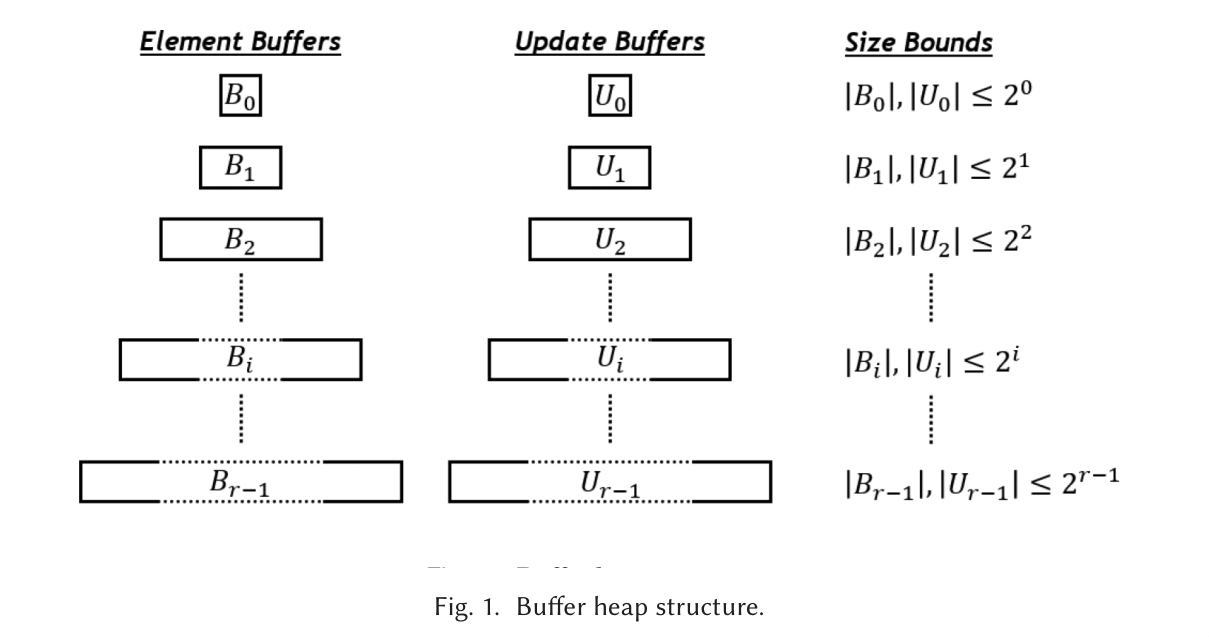
Figure 1: Screenshot from Chowdhury and Ramachandran (2018): the data structure has separate buffers for contained values and updates.
Either way the “technical overview” section in this paper is recommended reading: in-memory decrease-key solutions can keep a pointer, but this is not efficient in external memory. To identify the nodes for removal, two indices are needed, one by priority and one by ID, which is what complicates things in the first place. (I guess a general statement would be that it’s hard/impossible to store an arbitrary bijection in such a way that it can be updated and queried from both directions in \(O(\frac 1B)\) I/Os per operation.)
The technique of separately storing updates was also done before already.
The main layout is as follows: there are around \(\log n\) layers and layer \(i\) contains at most \(2^i\) elements and at most \(2^i\) updates (see the figure), such that all keys in layer \(B_i\) are less than those in layer \(B_{i+1}\). Furthermore, all updates to the elements in \(B_i\) that are not yet applied live in \(U_0, \dots, U_i\). Lastly, each \(B_i\) contains each id at most once, and buckets of elements and updates are sorted by id (rather than by key)! Updates are also sorted by timestamp as a secondary key in case multiple updates touch a single element. (Although, if the keys/priorities are (sufficiently) unique, sorting by that can surely also work.)
I’ll now briefly summarize the operations on the data structure. See the paper for more detail (where the full explanation, pseudocode, and analysis is a total of 10 pages).
Decrease-key simply pushes an update event to \(U_0\), and then fixes overflow of \(U_0\) if needed.
Sink. When \(B_{i-1}\) overflows, it is converted into a list of sink instructions that are merged into \(U_i\) (so that it remains sorted). Then once \(U_i\) is processed, this will add the element to \(B_i\).
Fixing \(U\) overflow is done by applying the updates of \(U_i\) to \(B_i\), emptying \(U_i\), and then moving remaining pending updates to \(U_{i+1}\). It recurses to larger levels \(i\) until \(U_i\) does not overflow anymore.
Apply-updates merges \(B_i\) and \(U_i\) and applies the necessary updates to each element, merging any extra updates into \(U_{i+1}\).
Delete-min and find-min first process updates coming before the first non-empty \(B_i\) and then also calling redistribute, which repeatedly partitions the smallest non-empty bucket into two halves (in this case, specifically in such a way that most buckets end up with exactly \(2^i\) elements).
Reconstruct is a function that is called after each operation and ensures the data structure remains in good shape. Specifically, if the data structure currently contains \(n\) elements, than this will force a rebuild of the entire structure once \(n/2\) operations are applied, so that the space overhead of pending deletes is never too large.
The main reason this has good I/O complexity is that updates are only gradually “pushed down” and merged into existing buffers. Furthermore, merging two buffers of \(2^i\) elements (or within a factor 2 of that or so) can be done for only a constant factor overhead in the I/O complexity.
2.3 Deletion tokens for the quickheap Link to heading
As with the buffer heap, our main idea is to insert the element with the new priority, and to insert a separate deletion token (anti matter) to indicate the element should be removed. So far, we assumed that the old priority is available when doing a decrease-key, so that we can directly push the deletion token to the right buffer rather than bubbling it down. We “clean up” a partition once $1/3$rd of it is deletion tokens. This operation entails finding matching elements and deletion tokens and this requires either hashing or sorting all elements. Neither is ideal, but it’s anyway inevitable, and so probably we should just sort the elements using an I/O-efficient (but not optimal) sort in \(O(\frac 1B \log_2 \frac nM)\) I/Os per element. Merge-sort already does this anyway.
One thing to figure out here is if pushing an update directly to the right bucket and only sorting that lazily later is bad. Currently I think it should be fine. If a bucket is cleaned up, should we also directly rebuild the entire subtree?
A specific difference is that in order to push an update to the right bucket, we need to know the old priority as an argument to the decrease-key call. The buffer heap paper does not assume this, and instead ’trickles down’ updates through the buckets.
2.4 Bloom filters Link to heading
Stefan Walzer also had an idea to use bloom filters to reduce the memory usage for cleaning up buckets with many deletions. First, we can build a, say, 8-bit filter on the deleted elements. Then we can scan through the elements and preserve those not in the filter. That should only leave a small fraction of elements that was false detected as deleted.
Then we can build an invertible bloom filter that also supports removing elements and looking up all elements contained in it, which has size proportional to the number of false-positive elements from before. Then we could insert all elements detected as deleted and remove all deleted elements, at which point we can read out the remaining elements.
This still uses \(O(n)\) space for a bucket of \(n\) elements, but it’s closer to \(n\) bytes rather than \(n\) words, which might make a difference in practice.
2.5 Counting bloom filters Link to heading
Another, more promising, idea (again by SW) to deduplicate buckets is the following: Create a counting bloom filter of, say \(n\) 8-bit counters. For each element, increment its corresponding counter, and for each delete, decrement it. Then filter out all the elements for which the counter is 0, since a count of 0 must mean all elements mapping to that counter have been deleted.
This leaves around false positives, in that some deleted elements map to a non-zero counter and are thus preserved, but that is OK: we can simply leave those in and filter them out the next time we deduplicate a bucket. If we use independent random seeds all should be fine as long as each iteration filters away at least a fixed fraction of the deleted elements. (This is unlike the bloom filter approach above, where the one-sided-probability was too eager in filtering out non-deleted elements, which needed an explicit second pass to resolve.)
It might already be sufficient to use 2-bit counters: we can first increment it for all inserts, and then decrement it for all deletes, but use the value 3 as ‘saturated’.
Either way, once all counters have been computed, we can compactify them into a 0/1-bitvector indicating which counters are positive and thus which elements should be preserved.
In case the counter vector would not fit in (small enough) cache, one option could also be to first pseudo-randomly (or by pivots?) partition the bucket into chunks that do fit in memory.
(Side question: why is it that partitioning into chunks feels very fast and I/O efficient, but hash tables are not I/O-efficient. I suppose partitioning is fast as long as each partition has at least \(\Omega(1)\) cache lines worth of data (as opposed to \(O(1/B)\) when accessing a single word). Thus, we could partition into \(O(M/B)\) blocks in one go? But then we get limited by the number of write-combining buffers probably.)
3 The SIMD radix heap Link to heading
Another idea is to combine the ideas of the SimdQuickHeap with the radix heap of Johnson (Johnson 1977). There are a few approaches to this: we can either radixify the quickheap, or simdfy the radix heap.
3.1 Adding SIMD to the radix heap Link to heading
This turns out to be not straightforward at all. Whereas the quickheap repeatedly partitions a layer into two, which can be done using comparisons and efficient compress-and-store SIMD instructions, the radix heap directly classifies elements into multiple groups, and SIMD scatter instructions aren’t nearly as efficient, and also require additional logic to make sure elements classified to the same bucket are written to consecutive (rather than the same) locations.
Either way, Patrick noticed that the C++ radix implementation that we use uses a loop to find the next empty bucket. Instead, we can simply keep track of which buckets are empty in a bitmask (see Marvin’s vibe-coded fork), which provides a decent (20%?) speedup. Additionally adding AVX-512 gave less of a benefit, IIRC.
3.2 Two-level radix heap Link to heading
The two-level radix heap is introduced by Ahuja, Mehlhorn, Orlin, and Tarjan (1990). A simple form is the following: instead of a radix of \(2\), use a first-level radix of say 4, so that elements are partitioned into \(w/2\) levels of how many trailing bits they share with the current minimum divided by 2 (for \(w=64\) bit values). Then, partition each level spanning \(4^i\) values into 4 segments by the top-2 bits of the value relative to the current minimum. This way, we first look the number of trailing zeros, and then at fixed number of bits before that. In a way, this is similar to floating point representations with an exponent and mantissa, but considering low-endian digits first.
The main benefit of this approach is that each partition step does not only use the number of trailing zeros, but also the last bits before that, so that overall, each element has to go through fewer partition operations, for less total I/O. In fact, this is similar to the multi-way partitioning we want to do for the quickheap as well.