- 1 Jaccard similarity
- 2 Hash schemes
- 2.1 MinHash
- 2.2 $s$-mins sketch
- 2.3 Bottom-\(s\) sketch
- 2.4 FracMinHash
- 2.5 Bucket sketch
- 2.6 Mod-bucket hash (new?)
- 2.7 Variants
- 3 Compressing sketches
- 3.1 $b$-bit hashing
- 3.2 HyperMinHash
- 4 Densification strategies
- 5 SimdSketch
- 6 Evaluation
- 6.1 Setup
- 6.1.1 Tools
- 6.1.2 Inputs
- 6.1.3 Parameters
- 6.1.4 Metrics
- 6.2 Raw results
- 6.3 Correlation
- 6.4 Comparison speed
- 6.5 Low-similarity data
- 6.1 Setup
- 7 Discussion
- 8 TODO / Future work
\[ \newcommand{\sketch}{\mathsf{sketch}} \]
This is a small survey on MinHash-based sketching methods, to go along with my
simd-sketch crate (github, crates.io, docs.rs). See also Cohen (2014) for a previous
small survey.
Goal. SimdSketch should be fast. It is and should remain a conceptually simple tool, that prefers fast implementations of simple ideas over complex ideas. For now, it works well for the simple case of relatively high identity sequences. I may implement more algorithmic variants, but also the API should remain concise.
Motivation. Suppose we have a large number \(r\) of sequences of length around \(n\), that we want to quickly compare. One way to do this is by sketching each genome into a much smaller representation, and then doing the \(\Theta(r^2)\) comparison only on the sketches.
Acknowledgements. This work was inspired by conversations with Karel Břinda, and improved by feedback from Jianshu Zhao.
1 Jaccard similarity Link to heading
Instead of comparing input sequences directly, we consider them as a set of k-mers (Heintze 1996). Then, the Jaccard similarity between two sets \(A\) and \(B\) is (Broder 1997; Broder et al. 1997) \[ \frac{|A\cap B|}{|A\cup B|}. \]
Thus, the goal is to estimate the Jaccard similarity via small sketches.
2 Hash schemes Link to heading
2.1 MinHash Link to heading
The first step is the simple MinHash (Broder 1997), that hashes all k-mers and selects the smallest hash value. The probability (over the random hash function) that sets \(A\) and \(B\) share the smallest k-mer equals the Jaccard similarity.

Figure 1: In this and the following figures, the horizontal bar indicates the real number line, and the dots indicate the hashes of the k-mers. The yellow dots are the selected hashes, and their values are shown in a square box. MinHash simply selects the smallest hash.
Algorithm. This is simple to compute by using a rolling minimum. On random data, we expect the minimum to only update \(O(\log n)\) times, so the branch-predictor can do a good job and this will be fast in practice.
2.2 $s$-mins sketch Link to heading
To better approximate the similarity, we can use multiple (\(s=4\) here) hash functions, and compute the fraction of hashes for which the minimal hash is identical (Cohen 1997; Flajolet and Nigel Martin 1985). (Note that other papers also use \(k\) or \(t\) for the size of the sketch, but I will stick to \(s\) to not confuse this with the k-mer length.)

Figure 2: Here, the $s$-mins sketch uses 4 different hash functions, and samples the smallest value returned by each hash.
Algorithm. We run the previous algorithm \(s\) times, for \(O(ns)\) total time.
There are multiple papers attributing this method to Broder (1997) and Broder et al. (1997), and then remark that \(O(ns)\) is slow. Neither of these two papers ever considers using more than one hash function. Instead both of them only talk about the fast bottom-\(s\) sketch discussed below, that is much faster.
Instead, using multiple hashes first appeared in Broder et al. (1998) and the following journal paper Broder et al. (2000).
Still, I am not yet aware of a bioinformatics tool actually implementing the $s$-mins sketch. Although it has been used for cardinality estimates (Flajolet and Nigel Martin 1985).
2.3 Bottom-\(s\) sketch Link to heading
A problem with using multiple hash functions is that this is slow to evaluate. Instead, bottom-hash can be used, where the smallest \(s\) values of a single hash function are taken (Heintze 1996; Broder 1997; Broder et al. 1997; Cohen 1997).
The sketch of \(A\cup B\) is then given by the smallest \(s\) values of the union of the sketches of \(A\) and \(B\), and \(|A\cap B|\) is the fraction of those smallest \(s\) values that are in both \(A\) and \(B\).

Figure 3: The bottom-(s) sketch samples the (s) smallest values returned by a single hash function. The dashed line is explained in the text below.
This method is typically attributed to Broder (1997) and Broder et al. (1997), but in fact, as they mention, the idea of sampling the bottom \(s\) values of a hash already appeared independently a year before in Heintze (1996). Compared to that earlier work, the main contribution of Broder (1997) is the formalization of the resemblance and containment metrics, and the formal relation to the Jaccard similarity.
The sketch of \(A\cup B\) is not the total number of distinct elements in the union of the sketch of \(A\) and the sketch of \(B\). When \(\sketch(A) = [0,2,4,6]\) and \(\sketch(B)=[1,3,5,6]\), we have \(\sketch(A\cup B) = [0,1,2,3]\) (rather than \([0,1,2,3,4,5,6]\)) and the size of the intersection is \(0\).
Mash is a tool that uses this bottom-\(s\) sketch, and they introduce the mash distance that estimates the mutation rate based on the Jaccard similarity.
Naive algorithm. This is where things get interesting. The usual/naive approach is to incrementally keep a set of the \(s\) smallest elements seen so far as a priority queue (max-heap). Where the rolling minimum gets a total of \(\ln n\) updates (in expectation, on random input), the bottom-\(s\) get \(s \ln n\) updates in total (Broder 1997; Cohen 2014): the \(i\)’th element has probability \(s / i\) of being in the bottom-\(s\), which sums/integrates to \(s \ln n\). Each update takes \(O(\log s)\) time, for overall complexity \(O(n + s\log s \ln n)\).
Better complexity (new?). We can do better by dropping the priority queue! Currently we do a bunch of ’early’ insertions into the heap of elements that will later be evicted. Instead, we can estimate the size of the largest value as \(T=s/n \cdot 2^{32}\) (for 32-bit hashes). Then, we can only insert elements up to, say, \(2T\) (indicated by the dashed yellow line). If there are a lot of duplicate-kmers, this may not be sufficient, and we can double the limit until \(s\) distinct hashes have been found. When there are no/few duplicate k-mers, this runs in \(O(n + s \log s)\).
Faster algorithm (new?). In practice, we can speed this up more: first collect all the values up to \(2T\), which can be done branchless and using SIMD, and then sort those in a separate pass. That way, the first loop over all \(n\) hashes can be completely branchless. See 5 for details.
2.4 FracMinHash Link to heading
This problem of the unpredictable threshold can also be solved by simply fixing the threshold (as the solid yellow line), and then taking however many hashes are below it. This is what fracminhash does (Irber et al. 2022).
This is also similar to mod-sketch that simply keeps all values \(0\pmod m\) for some modulus \(m\) (Broder 1997).

2.5 Bucket sketch Link to heading
Bottom-$s$-hash and fracminhash have the drawback that computing the similarity between two sketches requires a pass of merge-sort, which is hard to make efficient. Bucket-hash solves this by splitting the hashes into \(s\) buckets and returning the smallest hash in each bucket (Flajolet and Nigel Martin 1985; Li, Owen, and Zhang 2012).
This way, comparing two sketches is again as simple as computing the fraction of shared elements in equal positions.

Figure 4: The bucket sketch splits the output range of the hash function into (s) parts, and samples the smallest value in each part.
This scheme was introduced under the name one permutation hashing (Li, Owen, and Zhang 2012), but I think this is a bad name. In particular, the abstract of that paper writes:
Minwise hashing (Broder et al. 1998, 1997) is a standard technique in the context of search, for efficiently computing set similarities. […] A drawback of minwise hashing is that it requires a costly preprocessing step, for conducting (e.g.,) \(s=200\sim 500\) permutations on the data.
Indeed, the first cited paper introduces the $s$-mins sketch, but the bottom-\(s\) sketch already uses a single hash function and is much faster to compute. Indeed, the distinctive property of this one permutation scheme is not the fact that it uses only a single permutation/hash, but rather that it uses partitions/buckets to extract multiple smallest values.
Algorithm. This can be implemented by tracking \(s\) bucket values, and for each hash, comparing it with the current minimum in its bucket. This now requires \(n\) random memory accesses, and \(O(s \log s)\) writes. On the other hand, L1 cache can hold 4096 such values, and adjacent iterations can be mostly executed in parallel, so it may not be too bad.
2.6 Mod-bucket hash (new?) Link to heading
A drawback of bucket-hash is that computing it requires \(s\) ‘‘independent’’ minima. It’s not quite as bad as computing \(s\) hash functions, but it’s somewhat involved to compute (using SIMD instructions) whether an element is small within its bucket.
To fix this, we change the way we partition the data into buckets. Instead of linearly, we can split by the remainder modulo \(s\). That way, all selected elements will be small. In fact, the largest element will be around \(T=O(s \log s)\), and so we can pre-filter for elements up to \(2T\) (dashed line, again followed by doubling as long as needed).

Algorithm (new). To implement this efficiently, we can again collect small elements via a branchless SIMD implementation. Then we simply make a pass over those elements and update the minimum of each bucket.
A drawback is that there could possibly be empty buckets in unlucky cases. In that case, the threshold would be doubled until it reaches \(2^{32}\), and the pre-filter step becomes useless. But this should hopefully be rare.
2.7 Variants Link to heading
Instead of hashing all k-mers, it’s also possible to only hash the minimizers, as done by mashmap (Jain, Dilthey, et al. 2018) and fastANI (Jain, Rodriguez-R, et al. 2018).
Another variant is to apply the bottom-\(s\) sketch to only the k-mers with a hash \(0\bmod m\) (Broder 1997).
Another extension is to weighted input sets (multisets), e.g. Ertl (2018, 2020), where the number of times a k-mer appears affects the similarity.
3 Compressing sketches Link to heading
3.1 $b$-bit hashing Link to heading
So far, we have been storing full 32-bit hash values. We typically know the approximate size of the smallest elements, and thus, the high bits do not give much information. Thus, we can only store the low \(b\) bits of each hash value (Li and König 2010), for example only the bottom 8 bits of each 32 bit value, or even the bottom 1 or 2 bits only. As we will see, the sample size has to increase (by e.g. a factor \(3\)) to ensure the variance remains low, but overall this then still saves \(10\times\) over a 32-bit representation.

Figure 5: We can use the highest bits (black) to determine the bucket where the hash goes, and the lowest (b) bits (yellow) to determine the value stored in the bucket.

Figure 6: The same as before, but with mod-buckets we use the lowest bits to determine the bucket and we store the (b) bits just above that.
Apart from only being smaller, this also allows significantly faster comparison of sketches, since less data has to be processed.
A drawback is that after compression to the bottom \(b\) bits, sketches can not be merged, since there is no way to compare the missing high-order bits.
When \(b=1\), simple popcount instructions can be used to count the number of
equal bits in two sketches. When \(b\in\{8,16,32\}\), SIMD instructions can be
used to compare two vectors of integers.
For remaining values like \(b\in\{2,4\}\), a list of 64 values can be transposed and stored as \(b\) 64-bit values instead. Then after some xor and and/or instructions, a popcount can again count the number of equal values.
3.1.1 Accounting for collisions Link to heading
When \(b=1\), we expect half the bucket to match randomly. Similarly, when \(b=8\) we expect matches for \(1/256\) of the buckets.
Suppose the Jaccard similarity is \(x\). Then the probability that a bucket has matching values in two sketches is \[x’ := x + (1-x) \cdot 2^{-b}.\] We measure \(x’\), and would like to compute \(x\), so we invert this: \[x = (x’ - 2^{-b}) / (1-2^{-b}) = (2^b \cdot x - 1) / ( 2^b - 1).\]
3.2 HyperMinHash Link to heading
HyperMinHash (Yu and Weber 2017) (side note: this really is an excellent paper) combines techniques of HyperLogLog counters to achieve sketches with buckets of size \(O(\log \log n)\), rather than \(O(\log n)\). It still allows merging sketches and estimating cardinalities, which $b$-bit compression (see below) does not. The basic idea is that the probability that the minimum of a set is more likely to be small rather than large. If the minimum is large, the probability that the next-smallest number is only slightly larger is small, and thus, it is sufficient to only store the high order bits of each large number. Specifically, for each bucket one can use a floating point encoding with a 6-bit exponent and a 4-bit mantissa.
HyperMinHash is implemented in python in a corresponding github repo. A Go port is here (github) (called HyperMinSketch), and a Rust library based on that is here (github), which serves as the bases for a binary application, HyperMash (github). (The go port was also ported back to python (github).)

Figure 7: HyperMinHash uses the highest bits of a hash (black) to determine the bucket. It then stores the remainder of the hash in floating point/exponential notation: first the number of leading zeros (dashed arrow, the exponent), and then a few bits following the leading one (solid yellow line, the mantissa).

Figure 8: The same as before, but with mod-buckets: the low (b) bits are used to determine the bucket, and the value of remaining higher bits is encoded.
4 Densification strategies Link to heading
A drawback of bucket sketch is that some buckets can be empty when \(n\) not sufficiently larger than \(s\). A number of densification strategies have been proposed that ensure these buckets do not accidentally compare as equal, by filling them with k-mers from a different bucket.

Figure 9: Some buckets may be empty. What to do in that case? By default, we would simply store u32::MAX.
(Side note: I’m not convinced this densification matters all that much in practice. Usually when sketching, \(n\gg s\), and only very few buckets should remain empty?)
Rotation. A first option is to replace the value of an empty bucket by the (rotationally) next non-empty bucket (Shrivastava and Li 2014a).

Figure 10: Copying the value from the first non-empty right neighbour.
Random rotation direction. Instead of always picking the value of the next bucket, we can also choose between the previous and next bucket, via some fixed random variable \(q_i\in\{0,1\}\) that indicates the chosen direction (Shrivastava and Li 2014b).

Figure 11: Copying the value from either the left or right neighbour, determined by a pseudorandom hash of (i).
Still, for very sparse data the schemes above provide bad variance when there are long runs of empty buckets.
Optimal densification. A better solution is that every empty bucket \(i\) copies its value from an independent non-empty bucket \(j\). This can be done using a hash function \(h_i : \mathbb N \to \{0,\dots,s-1\}\) that is iterated until a non-empty bucket is found (Shrivastava 2017).

Figure 12: Optimal densification removes the correlation between adjacent empty buckets by letting each bucket have its own search (the dashed arrows) for a non-empty bucket to pull from.
Fast densification. It turns out the ‘‘optimal’’ densification strategy can be improved by using a slightly different algorithm. Instead of pulling values from filled buckets to empty bucket, filled buckets can push values into empty buckets (Mai et al. 2020). The authors shown that \(\lg s\) rounds of pushing values is sufficient, for \(s \lg s\) overall time.

Figure 13: When there are only very few filled buckets, searching for one can be slow. In that case, it’s faster to push from filled buckets to empty buckets: each bucket tries copying its value to empty buckets util all are filled.
Multiple rounds. All the methods so far suffer when, say, all k-mers hash to the same (or only very few) buckets. A solution is to use multiple hash functions (Dahlgaard, Knudsen, and Thorup 2017). As long as there are empty buckets, we do up to \(s\) rounds of re-hashing the input with a new hash \(h_i\). This is sufficiently fast in expectation, since it’s exceedingly rare to have empty buckets. If there are still empty buckets, we fall back to \(s\) hashes \(h’_i\), the $i$th of which maps all values into bucket \(i\), so that it is guaranteed each bucket will eventually be non-empty.

Figure 14: Still all these methods have high variance, since they only consider the set of bucket-minimal hashes. Instead, we can use multiple hash functions to fill non-empty buckets.
SuperMinHash does conceptually the same as the scheme above, but ensures that over the first \(s\) rounds, every element is mapped to exactly once to each bucket (Ertl 2017). This is done by explicitly constructing a permutation to control the bucket each element is mapped to in each round. However, this has expected runtime \(O(n + s \log^2 s)\).
ProbMinHash improves over SuperMinHash by tracking for each bucket the best value seen so far, and ensuring that for each element, the hash-values for each bucket are generated in increasing order (Ertl 2020). That way, the insertion of an element can be stopped early. It also provides a number of different algorithms for both unweighted and weighted sketching.
Skipping empty buckets (new?). One other, much simpler, option could be to detect when both
\(A\) and \(B\) have an empty bucket (i.e., when both store u32::MAX),
and then simply skip such buckets. My feeling
is that this should give unbiased results.

Figure 15: Instead, we can also store a bitmask that indicates the empty buckets.
5 SimdSketch Link to heading
SimdSketch currently implements the bottom-\(s\) and mod-bucket sketches, and support $b$-bit hashing for \(b\in\{32,16,8, 1\}\). It does not do any kind of densification.
In the implementation, we use the packed-seq crate to efficiently iterate over
8 chunks of a sequence in parallel using SIMD. We reuse parts of the
simd-minimizers crate for efficient ntHashing of the k-mers.
If we have a u32x8 SIMD element of 8 32-bit hashes, we can compare each
lane to the threshold \(T\). We efficiently append the subset of elements that are
smaller to a vector using a technique of Daniel Lemire.
6 Evaluation Link to heading
6.1 Setup Link to heading
6.1.1 Tools Link to heading
We compare SimdSketch BinDash (Zhao 2018; Zhao, Both, et al. 2024), which implements the bucketed version with $b$-bit hashing and optimal densification. It also supports multithreading. (The name stands for bin-wise densified minhash.) BinDash v2 adds support for additional densification techniques, and uses SIMD to speed things up.
We also compare against BinDash-rs (Zhao, Zhao, et al. 2024), which wraps the probminhash crate and implements a few of the algorithms of the ProbMinHash paper (Ertl 2020).
For both BinDash and BinDash-rs, we only use the default densification scheme, since in practice (at least for our use-case with \(n\gg s\)), densification does not matter much.
Further tools that we do not currently compare against:
Sourmash (Irber et al. 2024) is a software package that implements FracMinHash.
Dashing (v1, github, v2, github) (Baker and Langmead 2019; Baker and Langmead 2023) is based on HyperLogLog counters. To me, the only difference in the sketch compared to HyperMinHash mentioned above seems to be that it only stores the exponent part, and drops the mantissa. (The authors do cite the HyperMinHash paper, but never explicitly compare against it, so I’m not 100% sure.)
Setsketch (Ertl 2021) seems like a more complicated followup on probminhash and I haven’t properly read it yet. It also incorporates ideas of HyperLogLog into sketching. Feel free to reach out to give me the summary :)
6.1.2 Inputs Link to heading
We compare tools on 1000 sequences of Streptococcus Pneumoniae, downloaded from
zenodo (i.e., the first 1000 sequences in streptococcus_pneumoniae__01.tar.xz). Almost
all of them are close to 2 MB in size, with a few outliers up to 6 MB.
6.1.3 Parameters Link to heading
We sketch these inputs using the different tools and different methods. We vary the size (as in, number of elements) of the sketch as \(s\in\{128, 1024, 8192\}\). We use the bottom-\(s\) sketch with \(s=65536\) as a baseline for the Jaccard similarity, since computing exact k-mer sets is slow. The bit-width is \(b\in\{32,16,8,1\}\). (TODO: also support \(b=4\) and \(b=2\).)
For all experiments, we fix \(k=31\).
6.1.4 Metrics Link to heading
We compare methods on a few metrics.
- Time to sketch all 1000 input sequences.
- Time for each pairwise comparison, \(\binom{1000}2\) in total.
- The accuracy of the metric, as correlation with the baseline.
We do not compare the size of the sketch in itself, since it shouldn’t usually be a bottleneck. The main benefit of a small size is faster pairwise comparisons.
Note that we run tools on multiple threads when supported to speed up the evaluation, but all numbers are reported as CPU time. The CPU is an Intel i7-10750H, with the clock frequency fixed to 2.6 GHz and hyperthreading disabled.
6.2 Raw results Link to heading
| Tool | Sketch type | size \(s\) | $b$-bits | Sketching (s) | Distances (s) | Correlation |
|---|---|---|---|---|---|---|
| BinDash | bottom | 128 | 64 | 113.3 | 0.580 | 0.9669 |
| BinDash | bottom | 1024 | 64 | 116.3 | 3.580 | 0.9960 |
| BinDash | bottom | 8192 | 64 | 138.6 | 29.450 | 0.9994 |
| SimdSketch | bottom | 128 | 8 | 2.0 | 0.216 | 0.9655 |
| SimdSketch | bottom | 1024 | 8 | 2.0 | 1.699 | 0.9965 |
| SimdSketch | bottom | 8192 | 8 | 2.1 | 13.689 | 0.9993 |
| SimdSketch | bottom | 32768 | 8 | 2.8 | 54.954 | 0.9999 |
| BinDash | bucket | 128 | 1 | 124.7 | 0.270 | 0.8996 |
| BinDash | bucket | 128 | 8 | 124.7 | 0.250 | 0.9649 |
| BinDash | bucket | 128 | 32 | 124.6 | 0.240 | 0.9650 |
| BinDash | bucket | 1024 | 1 | 125.2 | 0.260 | 0.9864 |
| BinDash | bucket | 1024 | 8 | 124.9 | 0.300 | 0.9959 |
| BinDash | bucket | 1024 | 32 | 125.1 | 0.350 | 0.9959 |
| BinDash | bucket | 8192 | 1 | 126.4 | 0.370 | 0.9978 |
| BinDash | bucket | 8192 | 8 | 126.7 | 0.600 | 0.9994 |
| BinDash | bucket | 8192 | 32 | 127.1 | 1.740 | 0.9994 |
| BinDash-rs | bucket | 128 | 32 | 146.4 | 0.246 | 0.9588 |
| BinDash-rs | bucket | 1024 | 32 | 145.8 | 0.353 | 0.9929 |
| BinDash-rs | bucket | 8192 | 32 | 147.1 | 1.977 | 0.9987 |
| SimdSketch | bucket | 128 | 1 | 2.0 | 0.005 | 0.9254 |
| SimdSketch | bucket | 128 | 8 | 2.0 | 0.014 | 0.9677 |
| SimdSketch | bucket | 128 | 16 | 2.0 | 0.015 | 0.9677 |
| SimdSketch | bucket | 128 | 32 | 2.0 | 0.015 | 0.9678 |
| SimdSketch | bucket | 1024 | 1 | 2.0 | 0.011 | 0.9861 |
| SimdSketch | bucket | 1024 | 8 | 2.0 | 0.057 | 0.9945 |
| SimdSketch | bucket | 1024 | 16 | 2.0 | 0.065 | 0.9945 |
| SimdSketch | bucket | 1024 | 32 | 2.0 | 0.067 | 0.9944 |
| SimdSketch | bucket | 8192 | 1 | 2.2 | 0.035 | 0.9977 |
| SimdSketch | bucket | 8192 | 8 | 2.2 | 0.382 | 0.9994 |
| SimdSketch | bucket | 8192 | 16 | 2.2 | 0.595 | 0.9994 |
| SimdSketch | bucket | 8192 | 32 | 2.2 | 0.881 | 0.9994 |
| SimdSketch | bucket | 32768 | 1 | 3.0 | 0.110 | 0.9996 |
| SimdSketch | bucket | 32768 | 8 | 3.0 | 1.736 | 0.9999 |
| SimdSketch | bucket | 32768 | 16 | 3.0 | 2.788 | 0.9999 |
| SimdSketch | bucket | 32768 | 32 | 3.0 | 4.074 | 0.9999 |
| SimdSketch | bucket | 131072 | 1 | 6.9 | 0.541 | 0.9999 |
The table above compares all tools. Some observations:
- The time for sketching is mostly independent of the input parameters, since the hashing of k-mers is the bottleneck. (Only the size \(s=8192\) sketch is slighly slower at times.)
- SimdSketch is significantly faster with sketching: both the bottom and bucket variant take around 4 s, while BinDash takes at least 118s (\(30\times\) slower) and BinDash-rs at least 145 s (\(36\times\) slower).
- Computing distances is faster when \(s\) is small, and faster when \(b\) is small, since there is simply less data to process.
- SimdSketch is around \(2\times\) faster than BinDash when comparing bottom sketches. But note that this is slow compared to bucket sketches.
- BinDash-rs has comparable comparison performance to BinDash.
- SimdSketch is well over \(10\times\) faster at comparisons in most cases. For a part, this is likely due to having all sketches in memory, rather than reading them from disk as BinDash does. But BinDash-rs is also fully in memory, and just slower for some reason.
- For $b$-bit variants, storing only the 8 bottom bits is as good as storing the full 32 bits, and is faster to compare. Using only the bottom 1 bit is faster still (especially for SimdSketch), but correlation goes down, which would have to be compensated by a larger sketch size.
6.3 Correlation Link to heading
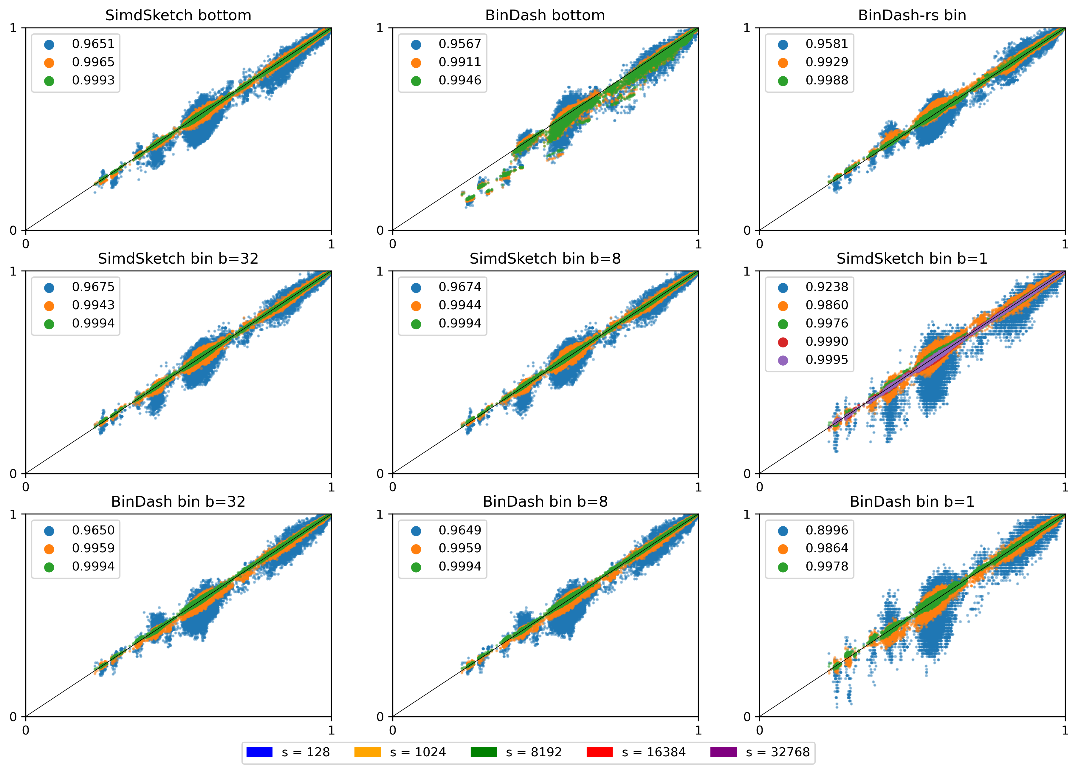
Figure 16: (Click to open in a new tab.) Correlation between the similarity reported by each scheme and the (s=65536) bottom-sketch. Colours indicate the value of (s), and legends show the correlation. Note that this compares purely the estimated Jaccard similarity between k-mer sets. Conversions to reporting ANI or mutation rate have been removed.
The top row shows the two bottom variants, and BinDash-rs. The middle row shows SimdSketch for varying \(b\), and the bottom row shows BinDash for varying \(b\).
Again some observations:
- Larger \(s\) gives better results: the spread of the green points is much less than orange and blue.
- BinDash and SimdSketch give very similar results for the bucket hash (middle and bottom row), and also very similar to BinDash-rs (top right).
- \(b=8\) (middle column) looks very similar to \(b=32\) (left column). \(b=1\) is worse.
- Fixed by now: BinDash’s bottom sketch (middle top) was off (github issue).
6.4 Comparison speed Link to heading
We now look slightly closer at comparing the speed of comparing sketches, versus the correlation this gives.

Figure 17: Log-log plot comparing the throughput of comparing sketching (in millions per second, larger/more to the right is better) to how close the correlation is to (1) (more to the top is better). Colours indicate the tool and variant (bottom soft circles, buckets bright crosses). Larger icons correspond to larger sketches (larger (s)). Solid lines connect data points that only differ in the choice of (s), and dashed lines connect points that only differ in (b).
We see that bottom sketches are significantly slower to compare than bucket sketches. BinDash (blue) is slightly faster than BinDash-rs (black), but SimdSketch (red) is significantly faster than both.
The highest throughput is obtained when \(b=1\) (the rightmost solid line). Larger \(s\) give better correlation (higher dashed lines / larger crosses). Specifically for \(b=1\) we added some data points with even larger \(s \in \{16384, 32768\}\), and we see that these outperform \((b, s)=(8, 8192)\).
6.5 Low-similarity data Link to heading
Here we consider a different dataset, with much lower similarities: a collection of bacterial genomes (Streptomycetaceae), downloaded using genome updater:
| |
We use the fist 1072 sequences (of ~11k total). These are around 8Mbp each.
We make a similar plot to before, but now use slightly larger sketch sizes and include \(b=16\).
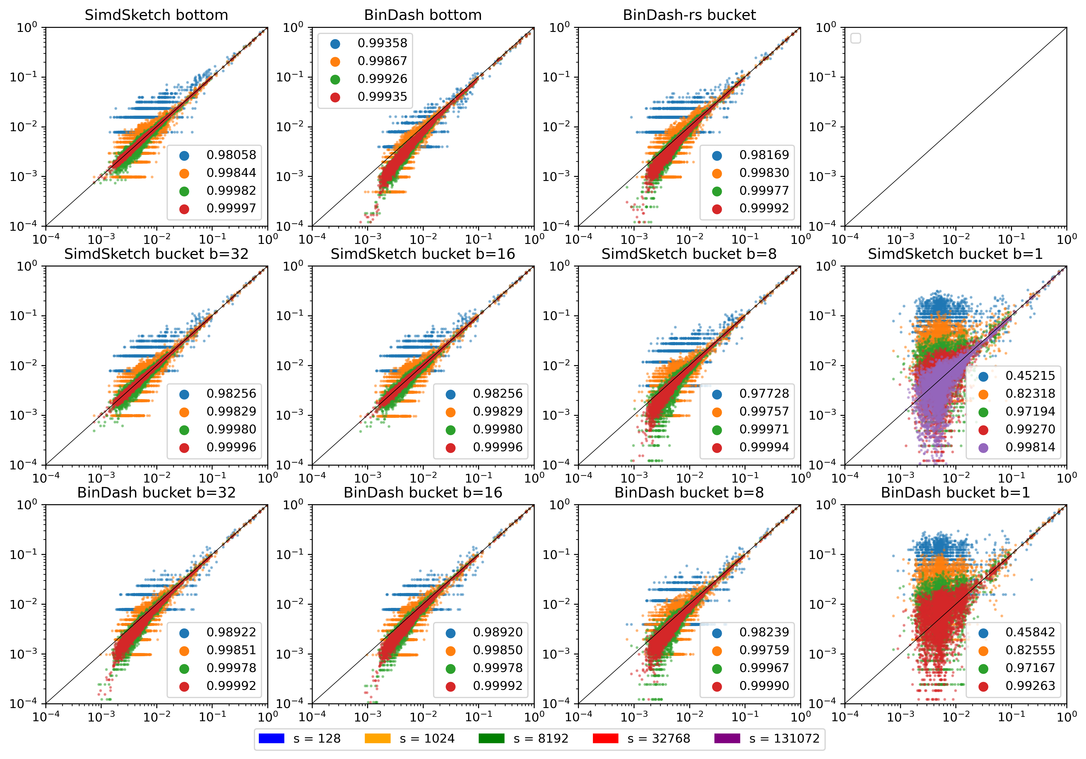
Figure 18: (Click to open in a new tab.) Log-log plot of correlation between the similarity reported by each scheme and the (s=65536) bottom-sketch. Colours indicate the value of (s), and legends show the correlation. Note that this compares purely the estimated Jaccard similarity between k-mer sets. Conversions to reporting ANI or mutation rate have been removed.
There is a lot of weird stuff going on here:
- The SimdSketch bottom sketch has good correlation, as it is benchmarked against itself.
- SimdSketch bucket sketch:
- Good correlation for \(b=16\) and \(b=32\).
- For \(b=8\), our bucket sketch is some bias for small similarities. I’m not quite sure what is causing this. It could be that we wrongly correct for the \(1/256\) probability of bucket collisions, but I don’t think that’s the case.
- For \(b=1\), the results are simply too noisy. But there does not appear to be a bias, unlike for \(b=8\).
- BinDash bottom sketch:
- There is again some bias for small similarities. Maybe this is the same bug in BinDash as before, where the merge sort is not stopped early?
- BinDash-rs also has a similar bias. I’m unsure why.
- BinDash-rs bucket sketch:
- \(b=16\) or \(b=32\): There really should not be any bias here. I’m so confused why these results differ from SimdSketch.
- \(b=8\): The bias in the opposite direction (overestimating the similarity) is caused by the lack of correction for colliding buckets.
- \(b=1\): Again, simply too noisy.
A bug? I wonder if there is a mistake in both my bottom and bucket sketch, but that would very much surprise me. On the other hand, the BinDash bottom and bucket sketches seem to be in agreement with each other as well. Maybe instead I made a bug when modifying the code to report Jaccard similarity instead of ANI? But I just return the fraction of equal-valued buckets, with the correction applied. Or maybe it’s because I’m using 32-bit hashes?
Hypothesis. For \(b=8\), the probability of hash collisions is not actually \(1/256\), since the distribution of values is not uniform, but rather geometric/exponential. This could explain the weird results for \(b=8\), but not elsewhere.
As a sanity check, the bottom-\(s\) similarity between the $31$-mers of two random sequences of length 8 million is around 0.001, while the uncorrected bucket similarity is 0.004. After correction, though, that goes down to pretty much 0, and sometimes even negative?? Both these numbers are far off 0.001.
Or maybe the issue is collisions in the 32-bit hashes? We actually expect very few (basically no) matches between two random sets of 31-mers, yet this returns 0.001.
To be continued…
7 Discussion Link to heading
To summarize, SimdSketch is significantly faster than BinDash and BinDash-rs: around \(30\times\) for sketching with similar parameters, and at least \(4\times\) faster when comparing sketches at equal correlation, by using \(b=1\) and increasing \(s\).
When the number of sequences \(r\) is small (say \(\leq 5000\)), one should probably use e.g. \(s=8192\) and \(b=8\), since increasing \(s\) up to this point barely affects the time needed for sketching, and comparing sequences is not a bottleneck in this case. Storing only the last \(b=8\) bits has nearly no loss in performance compared to storing the full \(b=32\) bits, while being \(2.5\times\) faster.
When \(r\) is large (say \(\geq 50\ 000\)), it pays off to spend slightly (\(20\%\)) more time on the sketching by using \(s=32\ 768\) instead, of which we then only store the bottom \(b=1\) bit of each hash. This way, sketches are much smaller, and comparing sketches is \(4\times\) faster than before.
TODO 8 / Future work Link to heading
- Implement HyperMinSketch, basically storing the exponent and the high \(b\) bits of the mantissa of each hash, rather than the low \(b\) bits.
- Implement some densification strategies, just for testing.
- Implement the ‘skip’ densification strategy by storing a bit-vector of empty buckets.
- Benchmark on some low-identity data where the Jaccard similarity is as low as 0.001.
- Compare against dashing and/or HyperMinHash?