This post build on top of our recent preprint Groot Koerkamp and Ivanov (2024) and gives an overview of some of my new ideas to significantly speed up exact global pairwise alignment. It’s recommended you understand the seed heuristic and match pruning before reading this post.
Two subsections contain ideas that I haven’t fully thought through yet but sound promising1.
Motivation Link to heading
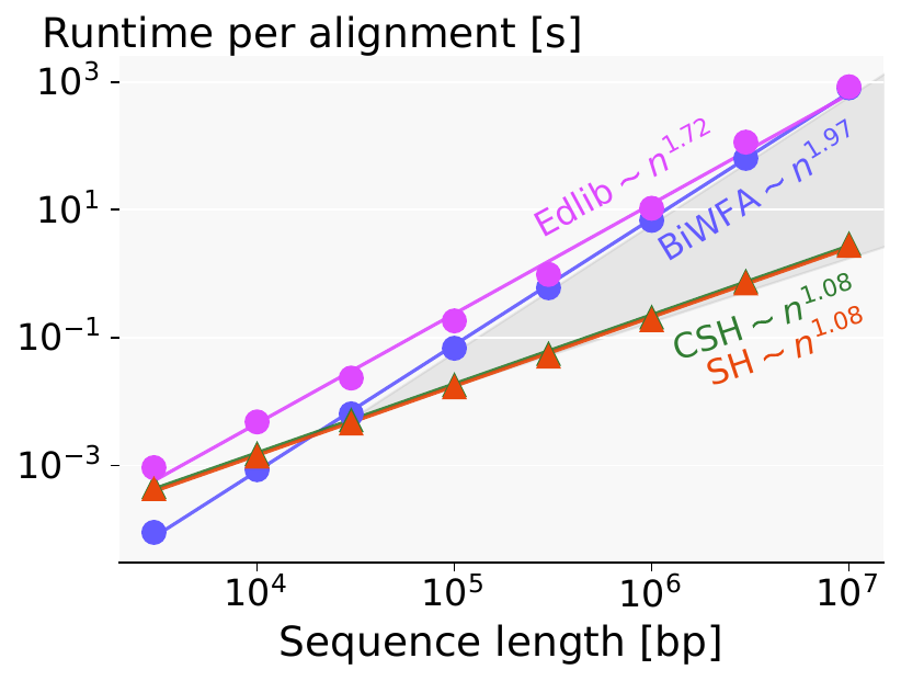
Figure 1: Figure 4b from our preprint: at (e=5%) error rate, the seed heuristic (SH) only outperforms BiWFA from (n=30kbp) onward.
In the preprint, we present an algorithm with near-linear runtime on random sequences. However, despite its linear runtime, it only outperforms BiWFA and Edlib for sequences with length \(n\geq30kbp\), due to the bad constant in the complexity. As a quick comparison, BiWFA and A*PA have similar runtime at \(n=30kbp\), \(e=5\%\) (Figure 1). BiWFA, with complexity \(O(s^2)\), needs to do \[ s^2 = (e\cdot n)^2 = (0.05\cdot 30\ 000)^2 = 1500^2 = 2.25M = 75 \times n\] operations. Conclusion: the constant of our \(O(n)\) A*-based algorithm is \(75\) times worse than that of BiWFA. Plenty of headroom for optimizations.
Summary Link to heading
The method I present here needs a candidate alignment \(\pi\) of cost \(t\) as input. It may be found via any approximate alignment method. Especially when \(\pi\) happens to already be an optimal alignment this new method should be an efficient way to prove that \(\pi\) is optimal indeed.
Instead of match-pruning the heuristic on the fly, we path-prune the the matches on \(\pi\) up-front. Then, instead of doing A*, we do WFA, but only on those states that satisfy \(f(u) = g(u) + h(u) \leq t\). The simplest way to do this is to simply trim from the ends of each wavefront states with \(f(u) > t\).
Why is A* slow? Link to heading
Even though our implementation uses \(O(1)\) datastructures for the things it needs to do (i.e. a bucket queue and hashmap), that does not mean these operations are actually fast.
In general, the A* has to do a lot of work for each processed state.
- compute \(h\) for each expanded and explored state;
- push and pop each state to/from the priority queue;
- store the value of \(g\) of each state in a hashmap.
Individually, these may not sound too bad, but taken together, the algorithm has to do a lot of work per state.
SIMD. Another reason A* is not fast is because none of it parallelizes well in terms of SIMD and instruction-pipelining2. Only one state can be processed at a time (assuming single-threaded code), and all the intermediate datastructures prevent looking ahead.3
WFA and Edlib on the other hand are DP based algorithms that benefit a lot from SIMD. In WFA, each furthest reaching point in wavefront \(W_{i+1}\) can be computed from wavefront \(W_i\) independently using equivalent and simple formulas – perfect for SIMD.4
Memory locality. This also has do to with memory locality: A* jumps all over the place in unpredictable ways, whereas WFA processes the input in a completely predictable way. Processors are good at processing memory linearly and have to resort to slower (L2/L3) caches for random access operations. Again this does not work in our favour.5
Computational volumes Link to heading
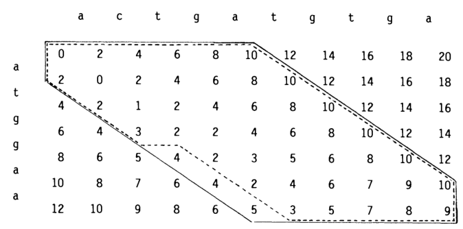
Figure 2: Figure from Spouge (1989). The dotted line shows a computational volume in the dotted where (g(u) + h(u) leq 13), where (g) are the numbers as shown, and (h) is (2) per indel needed to get to the end.
We have to do less and more predictable work.
A first step towards this are computational volumes (Spouge 1989), see Figure 2. Let’s assume we already know the length \(s\) of the optimal path. Then A* will expand all states \(u\) with \(f(u) = g(u) + h(u) < s\), and some states with \(f(u) = s\). It would be much more efficient to simply process exactly these states in order. That’s actually pretty straightforward: we can simply process them column-by-column (or using WFA) and filter out states where \(g(u) + h(u) > s\).
Precomputing front boundaries. We can save more time by not evaluating \(h\) in every state, but only in those on the boundary (top/bottom states) of the column (or wavefront): the boundary of the next column will be similar to the boundary of the current column, so we can first determine those and then fill the interior using standard SIMD-based methods.
Testing \(\leq t\). More generally, we can run this without knowing the actual distance \(s\), but for any test value \(t\). When \(t<s\), the computational volume will not include the end and we can rerun with increased \(t\). When \(t>s\), the right answer will be found, at the cost of increasing the width of the volume by roughly \(t-s\) on each side.
Order of computations. One we determine which states need to computed, we can compute them in any order we like:
- row/column-wise,
- anti-diagonal-wise,
- order of \(g\) (as in Dijkstra and WFA),
- order of \(f=g+h’\) (as in A*), where \(h’\) can be a different heuristic than the one used before.
For now my feeling is that option 3 is the fastest, but option 4 (in particular WFA with gap-cost) may need some investigation as well.
Dealing with pruning Link to heading
So, this is all nice, but actually our linear runtime heavily depends on pruning. Without pruning we inevitably get a ‘blow-up’ (Dijkstra-like behaviour) around the start of the search, where the band increases by \(1\) for each error not predicted by the heuristic.
A match is pruned once the state at its start is expanded. After pruning, the heuristic typically increases for most states preceding the match. When processing states column-by-column, this means that all states that could have been skipped because of pruning have already been computed anyway. The solution is to prune matches right from the start: path-pruning.
Assume we already have a candidate alignment \(\pi^*\) of cost \(s\). For now, let’s additionally assume that \(\pi^*\) is an optimal alignment, as indicated by the \({}^*\).
From \(\pi^*\), we can infer the distance \(g(u)\) to each state \(u\) on \(\pi^*\). Now, go though the matches on \(\pi^*\) in reverse order (starting at the end), and prune each match (starting at \(u\)) for which \(f(u) = g(u) + h(u) < s\).
After this process, the value of \(f\) anywhere on \(\pi^*\) will be at most \(s\).6 Note that \(f\) may be less than \(s\), and can go down from \(s\) to \(s-1\). This means that \(h\) is not consistent anymore, but that will not be a problem since all we need is admissibility (\(h(u) \leq h^*(u) = d(u, v_t)\)), which still holds7.
Now, we have a fixed (as in, not changing anymore because of pruning) heuristic, and we can apply the computational volumes technique from the previous section again.
If \(\pi^*\) is indeed an optimal path, this will efficiently prove that indeed \(\pi^*\) is optimal.
When \(\pi\) is not optimal (we drop the \({}^*\) from the notation), let’s assume it has cost \(t\), while \(s\) is still the optimal cost. We constructed \(f\) to take values up to \(t\), and so our heuristic definitely is not admissible anymore. However, in this case \(h\) will overestimate the true distance to the end \(h^*\) by at most \(e:=t-s\).8
The bandwidth condition of Harris (1974)9 tells us that when \(h\) overestimates \(h^*\) by at most \(e\), A* is guaranteed to find a shortest path after expanding all states with \(f \leq s + e = t\).10 Thus, the previous algorithm still works, even when the path \(\pi\) is not optimal!
Thoughts on more aggressive pruning Link to heading
This subsection is speculative.
Full pruning. Maybe it’s even possibly to path-prune all matches on the guessed path. That makes the heuristic inadmissible, but my feeling is that as long as we make sure to expand the start of all pruned matches at some point, this still works. Proof needed.
In combination with the front-doubling approach below, this could have the additional benefit that no initial path/cost estimate is needed.
I’m not quite sure whether this actually makes sense though. After pruning all matches on the path there is nothing to guide the heuristic anymore. The search will still be pushed towards the tip, but the tip will not be pulled across long indels.
Algorithm summary Link to heading
- Input
- Some alignment \(\pi\) of cost \(t\).
- Output
- An optimal alignment \(\pi^*\) of cost \(s\leq t\).
- Algorithm
- Construct the (chaining) seed heuristic \(h\).
- Compute \(g(u)\) for all states on \(\pi\).
- In reverse order, remove from \(h\) all matches (with start \(u\)) on the path \(\pi\) with
\(f(u) = g(u) + h(u) < t\).
Note: this pruning can be done directly during the construction of \(h\), since contours/layers in the heuristic are also constructed backwards. - Run your favourite alignment algorithm (Edlib/WFA), but after each front (ie column or wavefront), shrink the ends of the front as long as \(f(u) > t\) for states at those ends.
- When the algorithm finishes, it will have found a shortest path.
When the input \(\pi\) is optimal, this algorithm should have the complexity of A* (ie near-linear on random input), but the low constant of DP based approaches.
Challenges Link to heading
- When \(\pi\) overestimates the actual distance by \(e\), \(2e\cdot n\) extra work is done, since the computational volume increases in width.
- A good candidate \(\pi\) needs to be found. This could be done by finding the longest chain of matches in \(h\) and filling in the gaps using a DP approach, or by running a banded alignment algorithm.
- Computing \(h\) requires building a hashmap of kmers (or a suffix array). While that is relatively fast, it can in fact become the bottleneck when the rest of the algorithm is made more efficient. We’ll have to see how this ends up after doing experiments.
- It could happen that there are two good candidate alignments that are far from each other. In this case we should split each front (column/wavefront) into two smaller intervals of states \(f\leq t\) that cover the good candidate states, and skip the states in the middle with \(f > t\).
Results Link to heading
For now, I only did one small experiment on this where I compared A*PA to a non-optimized (read: very slow) implementation of WFA with a path-pruned heuristic, and the WFA version was \(3\) times faster that the A* version. I expect my WFA implementation to improve at least \(10\times\) after I optimize it for SIMD, so this sounds promising.
What about band-doubling? Link to heading
In Ukkonen (1985) and Edlib (Šošić and Šikić 2017), the band-doubling approach is used to find \(s\), instead of an oracle/test-value \(t\). This works by first testing \(t=1\), and then doubling \(t\) as long as testing \(t\) does not give an answer (i.e. \(t<s\)). This approach finds the right distance \(s\) with optimal complexity \(O(ns)\). The reason for this is twofold:
- Iterations with too small \(t<s\) do not add a significant overhead because of the exponential growth of the band: \(1+2+4+\dots+2^k < 2^{k+1}=t_{final}\).
- The final iteration (the first with \(t_{final}\geq s\)) has \(t_{final}\leq 2s\), which again has only constant overhead over \(s\).
Sadly, the same idea does not work as well when using a heuristic: When \(h\) is a perfect heuristic, testing \(t=s\) takes \(O(n)\) time. When doing $t$-doubling again, suppose that \(t=s-1\) failed. Then, we test \(t=2s-2\). This increases the number of computed states to \(2(t-s) \cdot n \approx 2s\cdot n\). When \(s\) is large and grows with \(n\), this is quadratic instead of linear!
Maybe doubling can work after all? Link to heading
This subsection is speculative.
NOTE: I have now written a dedicated post about this here.
Front-doubling. I’m thinking that maybe band-doubling can still work in a different way: Instead of doubling a global parameter, we double the size of each front (column/wavefront) whenever it needs to grow. But each front depends on previous fronts, so they need to grow as well to be able to compute the new front. Now, instead of a global threshold \(t\) we have a threshold \(t_\ell\) for each front \(\ell\).
Let’s assume that the size of a front roughly corresponds to the difference between the smallest and largest value of \(f\) of states in the front.11 Then, one way to double the size of a front is to double this difference:
- Let \(f_{min, \ell}\) be the minimum value of \(f\) in front \(\ell\). The maximum value is \(t_{\ell}\) by construction.
- Extend this and previous front up to \(f\leq t_\ell + t_\ell - f_{min,\ell} = 2t_\ell-f_{min,\ell}\). Thus, set \(t_{\ell’} = \max(t_{\ell’}, 2t_\ell - f_{min,\ell})\) for all \(\ell’ \leq \ell\).
- For each previous front \(\ell’\) that grows, make sure that its size (difference between \(t_{\ell’}\) and \(f_{min, \ell’}\)) at least doubles. If not, further increase \(t_{\ell’}\) and additionally increase \(t\) for previous fronts.
Now, this should12 guarantee that each front at least doubles in size.
To implement this, we keep all fronts in memory and simply grow them whenever needed.
And pruning? I think this can also work with a path-pruned heuristic, but we need to be careful since \(h\) is not consistent. That means that after growing a front, we may need to update already computed states of next fronts. But since we make sure to at least double the size of each front, just recomputing the entire next front doesn’t hurt the complexity.
I’m also hopeful that a fully path-pruned heuristic (i.e. with all matches on the path removed) can work here. The most important requirement is that we need to make sure that eventually all states at the start of a pruned match are indeed expanded. Otherwise it wouldn’t have been allowed to prune the match at all.
Maybe a middle-ground between online and path-pruning is possible: Once a path to a match has been found, we prune it from that point onward. For all future band-doublings we will take into account the pruned match. A drawback here is that the pruning only happens after the current doubling of the band. This means we compute too many states. But maybe since we’re only doubling on each iteration everything is fine. Again, experiments needed.
TODOs Link to heading
- Write down the proofs that are omitted here.
- Argue more formally where A* is slow.
- A more efficient implementation of WFA with heuristic is needed. Either I need to improve my own Rust implementation, or I need to path it into WFA directly.
- When that’s available, proper experiments need to be done with different approximate alignments \(\pi\).
- The time spent in various parts of the algorithm needs to be analysed.
- We can efficiently proof the correctness of candidate alignments, but do people care?
- Write a paper. (Current ETA: Q1'23. Help with coding it is welcome.)
Extensions Link to heading
- It may be possible to use this with BiWFA, when the heuristic is used on both sides.
- Instead of doubling \(t\), we could double the band when \(t\) is too small. That way, we will never do more than twice (or maybe \(4\) times) the optimal amount of work. But it’s not clear yet to me in what ways doubling of band differs from increasing \(t\). This requires some more thought.
References Link to heading
More promising than the main text, in fact, because they do not depend on a given path as input. ↩︎
Verification needed ↩︎
I suppose it would be possible to expand a few states in parallel, but that does not sound fun at all. ↩︎
For linear and single affine costs, the bottleneck is actually the Extend operation. Thanks to Santiago for this insight. ↩︎
Again, verification needed. ↩︎
Proof needed. ↩︎
Proof needed. ↩︎
Proof needed. ↩︎
Amit Patel remarked on his site that this looked useful in 1997 but he has never seen it actually being used. A nice example of how maths may only become useful much later. ↩︎
Our \(e\) is the same as in Harris (1974). Our \(s\) is his \(f(p^*)\). ↩︎
Or maybe the difference between the smallest and largest \(g\) or \(h\)? Needs investigation. ↩︎
experiments needed ↩︎