We’ll prove that using the “faster” binary search algorithm (see 2.2) that tracks the LCP with the left and right boundary of the remaining search interval has amortized runtime
\[ O\Big(\lg_2(n) + |P| + |P| \cdot \lg_2(Occ(P))\Big), \] when \(P\) is a randomly sampled fixed-length pattern from the text and \(Occ(P)\) counts the number of occurrences of \(P\) in the text.
Thus, when searching for patterns that follow the same distribution as the input text, the performance of the faster search method is nearly as good as the LCP-based \(O(|P| + \lg_2 n)\) method when patterns have only few matches.
First some background.
1 Suffix arrays Link to heading
Suffix arrays were introduced by Manber and Myers (1993). A suffix array \(S\) of a text \(T\) of length \(n = |T|\) is a permutation of \([n]=\{0, \dots, n-1\}\) such that \(T[S[i]..] < T[S[i+1]..]\), that is, the suffixes are sorted by the order \(S\).
Given the suffix array, one can search for a pattern \(P\) of length \(|P|\), which returns the position \(p\) of the first suffix \(T[S[p]..]\geq P\).
In general, we are usually interested in the entire interval of suffixes \(S[l..r]\) that start with the given pattern. This can simply be done by using two independent searches, as so does not affect the theoretical complexity. But of course, in practice it’s more efficient to find both boundaries in one go.
2 Searching methods Link to heading
Manber and Myers introduce three methods to search the suffix array, all based on binary search.
2.1 Naive \(O(|P|\cdot \lg_2 n)\) search Link to heading
The naive method works using a simple binary search on the suffix array.
| |
The binary search needs at most \(\lceil \lg_2(n+1)\rceil\) iterations, and in each iteration the slowest operation is the comparison of the suffix \(M=T[S[m]..]\) with the pattern \(P\), which in the worst case compares \(|P|\) characters in \(O(|P|)\) time. Thus, the overall runtime is \(O(|P| \cdot \lg_2 n)\).
2.2 Faster \(O(|P|\cdot \lg_2 n)\) search Link to heading
One of the bad cases of the naive method above is that in each iteration, the entire pattern \(P\) is matched. As the remaining search interval \([l, r]\) narrows, the remaining suffixes get more and more similar to \(P\). In fact, once we know that the first \(c\) characters of \(L=S[T[l]..]\) match the first \(c\) characters of \(R=S[T[r]..]\), every remaining string in the interval also starts with these same first \(c\) characters, and so does \(P\). Thus, in the comparison of \(M=T[S[m]..]\) and \(P\), we can skip the first \(c\) characters.
In practice, we implement this by keeping the lengths1 \(c_l\) and \(c_r\) longest common prefix of \(P\) with \(L\) and \(R\), and skipping the first \(\min(c_l, c_r)\) character comparisons.
| |
In the worst case, this method is still \(O(|P| \cdot \lg_2 n)\), but it’s widely known that this method performs very well in practice, and can even be faster than the \(O(|P|+\lg_2 n)\) method below.
2.3 LCP-based \(O(|P| + \lg_2 n)\) search Link to heading
Now suppose that for every step in the binary search, we have already precomputed values \(x_l=LCP(L, M)\) and \(x_r=LCP(M, R)\). (This is possible in \(O(n)\) time and space using a bottom-up approach on the implicit binary search tree that contains around \(n\) nodes.)
Now assume that in a step of the binary search, we have \(c_l\geq c_r\). Again following the original paper, there are three cases, as they nicely illustrated.
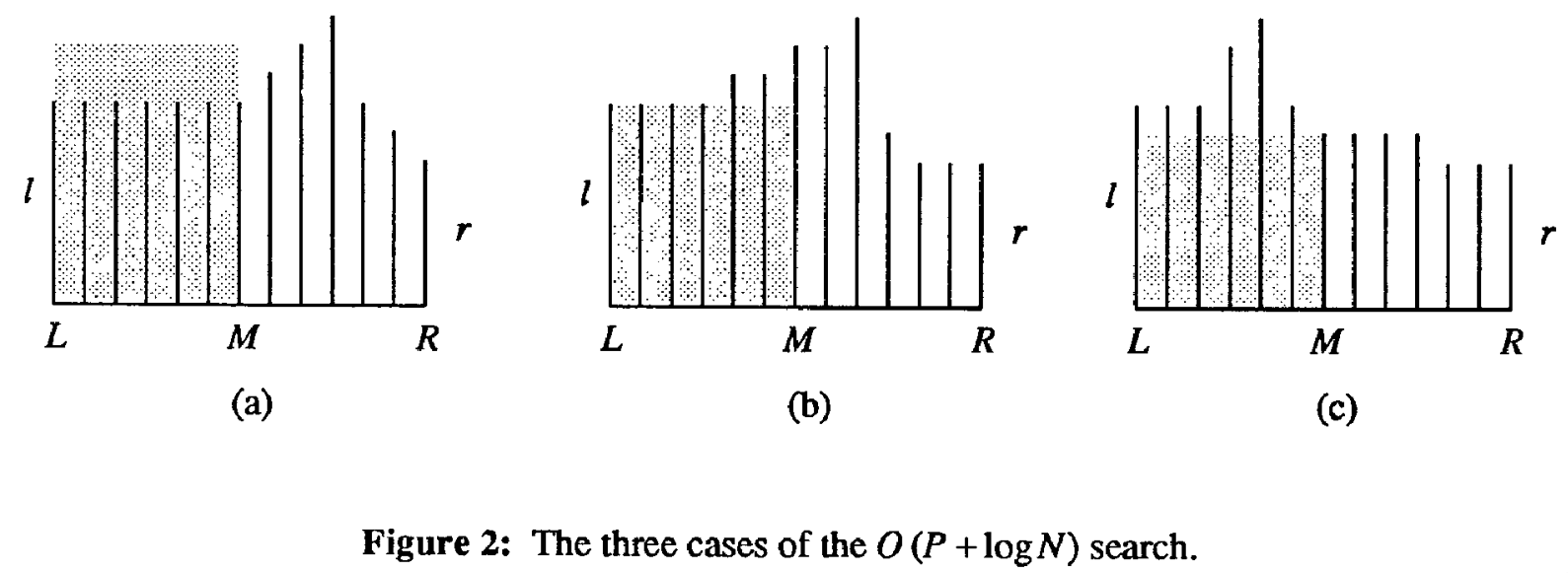
Figure 1: Three cases of the binary search, taken from Manber and Myers (1993).
The black bars indicate the length of the LCP of each suffix with \(P\), and \(c_l\) and \(c_r\) (\(l\) and \(r\) in the figure) are the length of the LCP of the left and right of the interval with \(P\). Assume that \(c_l\geq c_r\) (the symmetric case is equivalent). The grey area is the length of the LCP of \(L=T[S[l]..]\) and \(M=T[S[m]..]\).
Let \(x = LCP(L, M)\). The three cases are, in order:
- \(x > c_l\)
- In this case, we know that \(P\) is larger than \(L\) in the \(c_l+1\)‘st character, and since \(x>c_l\), \(L\) and \(M\) are equal in their \(c_l+1\)‘st character, so also \(P\) is larger than \(M\) in its \(l+1\)‘st character and \(P>M\), so we branch right.
- \(x=c_l\)
- In this case, we know that \(P\) shares the first \(x\) characters with \(L\) and hence also with \(M\). We now compare \(P\) with \(M\) starting at the \(c_l+1\)‘st character. Let’s say that \(h\) equal characters are compared. If we branch left, the new value of \(r\) is \(c_l+h\), and if we branch right, the new value of \(l\) is \(l+h\). Thus, \(\max(c_l, c_r)\) always increases from \(c_l\) to \(c_l+h\).
- \(x<c_l\)
- We know that \(P\) shares the first \(c_l\) characters with \(L\), and that \(L\) is less than \(M\) in its first \(x+1\leq c_l\) characters, so \(P<M\), and we branch left.
We see that the first and last cases take constant time, and since \(c_l\leq |P|\) and \(c_r\leq |P|\), we have \(\max(c_l, c_r)\leq m\). Since in the middle case the maximum is increased by \(h\). the total number of characters compared in case b. is at most \(m\). Thus, this method takes \(O(|P| + \lg_2 n)\) time.
3 Analysing the faster search Link to heading
The main difference between the faster search and the LCP based search is that the faster search starts comparing characters between \(P\) and \(M\) at the \(\min(c_l, c_r)+1\)‘st character, while the LCP version starts at the \(\max(c_l, c_r)+1\)‘st character. Thus, if we can show that the total number of compared characters ‘between’ \(\min(c_l, c_r)\) and \(\max(c_l, c_r)\) is not too large in expectation (in particular, at most \(|P|\)), we recover the expected runtime of \((|P| + \lg_2 n)\).
Let \(0\leq i\leq n\) be a uniformly random position in the text, and let \(P=T[i..i+m_P]\) be the pattern of length2 \(m_P\) starting at position \(i\). When \(i>n-m_P\), the pattern is simply a bit shorter than \(m_P\). In this case, we assume that \(P\) includes a sentinel character at the end, and thus will have exactly \(1\) occurrence in the text.
Consider a step in the binary search. We start comparing \(P\) and \(M\) at their \(\min(c_l,c_r)+1\)‘st character, and let \(y=LCP(P, M)\) be the computed length of the LCP of \(M\) and \(P\), which requires \(h=y-\min(c_l,c_r)\) comparisons of equal characters. We distinguish two cases:
- \(y < m_P\)
- When \(M\) does not start with \(P\), we know that the pattern is larger or
smaller than \(M\) with equal probability, since the pattern was randomly
sampled from the suffix array and thus each of the \(m-l\) position left of \(M\)
and each of the \(r-m\) positions right of \(M\) has an equal probability of corresponding
to the chosen pattern. (In the case where \(r-l\) is odd, we can randomly choose
between \(m=\lfloor \frac{l+r}2\rfloor\) and \(m=\lceil \frac{l+r}2\rceil\) to
equalize the probabilities.)
Thus, with probability \(1/2\), the minimum of \(c_l\) and \(c_r\) increases to \(y\), and so in expectation, the sum of \(c_l\) and \(c_r\) increases by at least \((y-\min(c_l,c_r))/2 = h/2\). Since the sum of \(c_l\) and \(c_r\) is at most \(2|P|\), the expected total number of comparisons is at most \(4|P|\).
- \(y = m_P\)
- When \(M\) starts with \(P\), we trivially do at most \(|P|\) comparisons. When there are \(Occ(P)\) occurrences of the pattern \(P\), this situation can happen at most \(\lg_2 Occ(P)\) times, and so this incurs a total cost bounded by \(O(|P| \cdot \lg_2 Occ(P))\).
We conclude that when we fix a length \(m_P\) and uniformly random choose a pattern \(P\) length \(m_P\) random from the input text, the amortized cost of a search is \[ O\Big(\lg_2(n) + m_P + m_p\cdot \lg_2(Occ(P))\Big). \]
References Link to heading
I’d like to use \(l\) and \(r\) here, but unfortunately they already indicate the left and right end of the search interval of \(S\). Sadly also \(l_\bullet\) for LCP length is already taken. ↩︎
I’m avoiding using \(m\) as the length of \(P\) since it’s also the position in the middle between \(l\) and \(r\) already. ↩︎