Range Minimum Queries
- 1 Naive
- 2 Space lower bounds
- 3 Sparse Table: \(O(1)\) queries, \(O(n \log_2 n)\) words
- 4 Segment Tree: \(O(\log n)\) queries, \(O(n)\) words
- 5 Blocks: \(O(s)\) queries, \(O(n/s \log n)\) words
- 6 Cartesian Trees: \(O(1)\) queries, \(O(n)\) words
- 7 Recursive Cartesian Trees: \(O(1)\) queries, \(2n+o(n)\) bits
- 8 Blackboard
\[ \DeclareMathOperator*{\argmin}{arg\,min} \newcommand{\rmq}{\mathsf{rmq}} \]
These notes are based on slides by Florian Kurpicz and the paper by Fischer and Heun (2011) that introduces a number of optimal implementations.
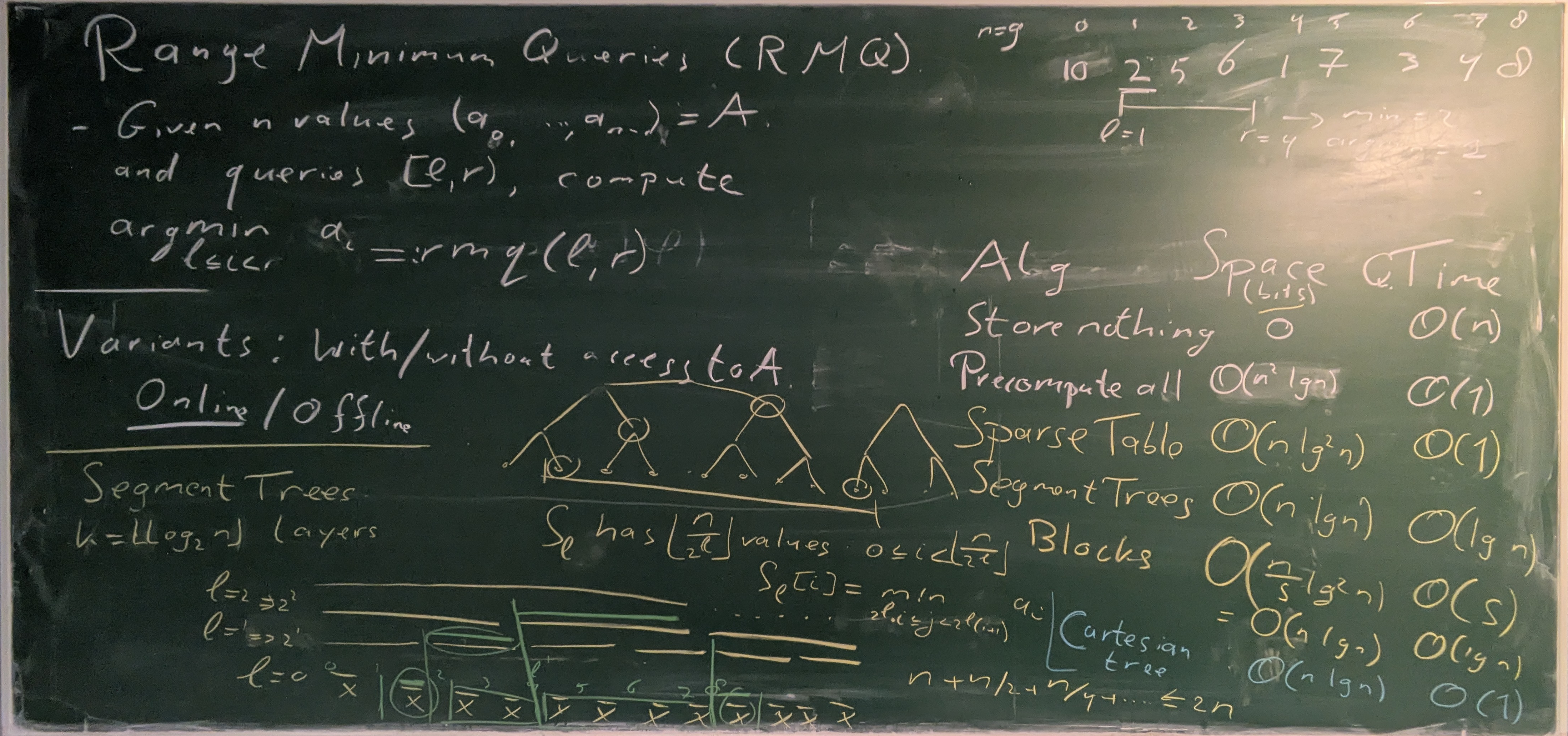
Given a list of \(n\) values \(A=(a_0, \dots, a_{n-1})\), build a data structure that can answer queries \([l,r)\) (\(0\leq l < r\leq n\)): \[ \rmq(l, r) = \argmin_{l\leq i< r}(a_i). \] Note that this returns the index of the minimum. For convenience, we assume throughout that ties are broken to the left (smaller index).
The goal is to have \(O(1)\) queries while using as little space as possible.
There are two variants:
- systematic schemes: where the data structure has access to \(A\), and
- nonsystematic schemes: where it does not have access to \(A\).
Additionally there is the offline setting where the queries are given in advance and can be processed as a batch. Here, we only consider the online setting.
One last remark is that the values \(a_i\) might take \(\omega(w)=\omega(\ln n)\) bits per element. For methods that normally store values \(a_i\) internally, a workaround is to compress the values into the range \([n]\) so that they can be stored in a single word.
1 Naive Link to heading
1.1 Compute on-the-fly Link to heading
The simplest option is to simply take \(A\), and answer all queries on-the-fly.
- Space overhead: \(0\).
- Query time: \(O(n)\).
1.2 Precompute everything Link to heading
A second option is to precompute all \(\binom{n+1}2\) answers \(\rmq(l,r)\). Since each \(\rmq\) value is between \(1\) and \(n\), they take \(\log n\) bits to store, regardless of the number of bits required by each \(a_i\).
- Space overhead: \(\binom{n+1}2 = O(n^2)\) words, or \(O(n^2 \log n)\) bits.
- Query time: \(O(1)\).
Note first that from here on, we will measure space overhead in bits, and second, that we will avoid using \(O()\) for the leading term.
2 Space lower bounds Link to heading
Before we continue, let’s consider space lower bounds, so we have an idea of how close to optimal the upcoming data structures are.
First, we show the following theorem (first stated in Jacobson (1989), who also introduced succinct data structures):
A nonsystematic data structure must use at least \(2n - \Theta(\log n)\) bits.
As a first note, we need at least \(n-1\) bits to store for each pair \((a_i, a_{i+1})\) whether \(a_i \leq a_{i+1}\) or \(a_i>a_{i+1}\), since this information is needed to answer queries \(\rmq(i, i+1)\).
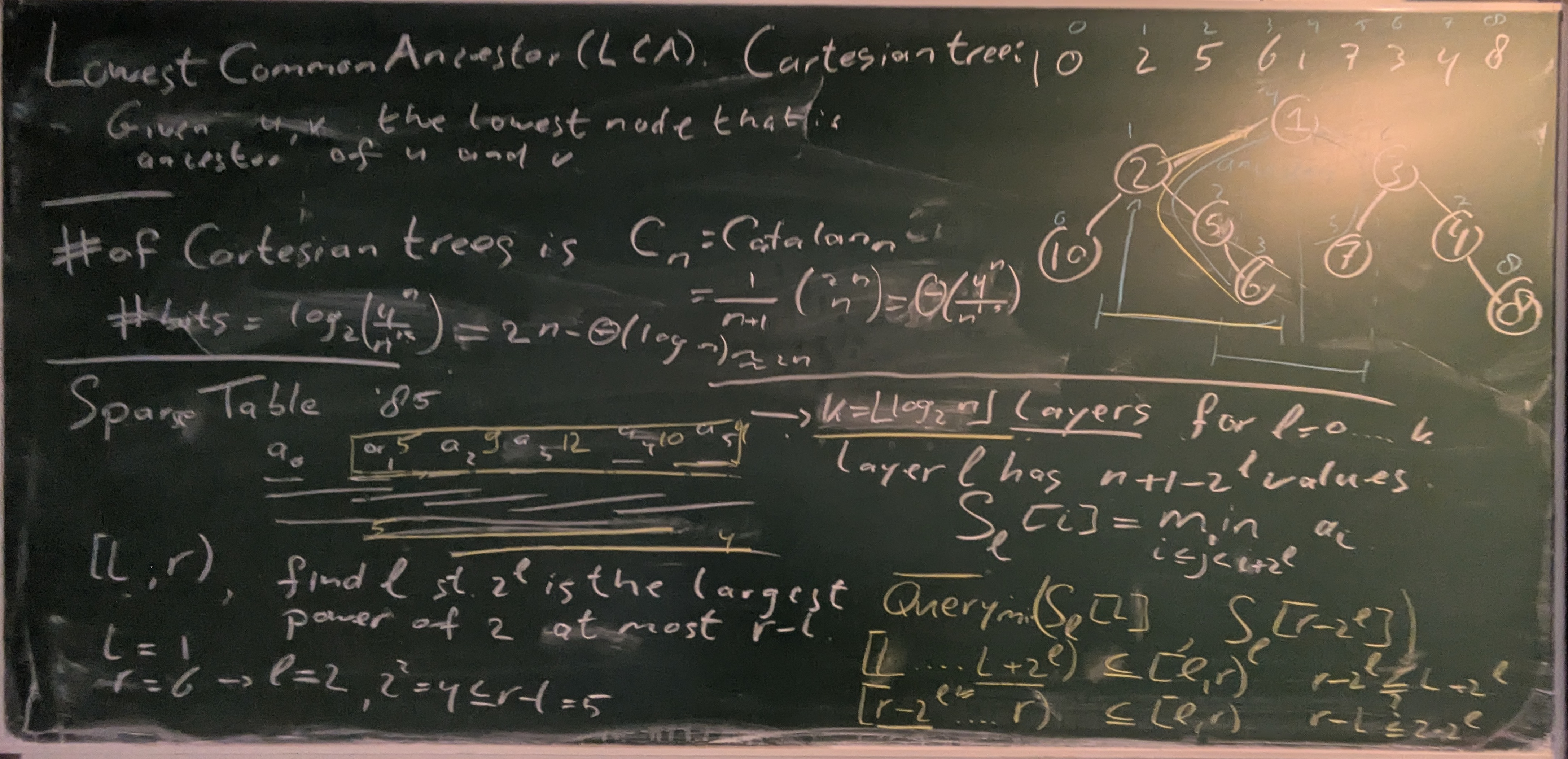
More generally, we can use the \(\rmq\) values to reconstruct the cartesian tree (wikipedia):
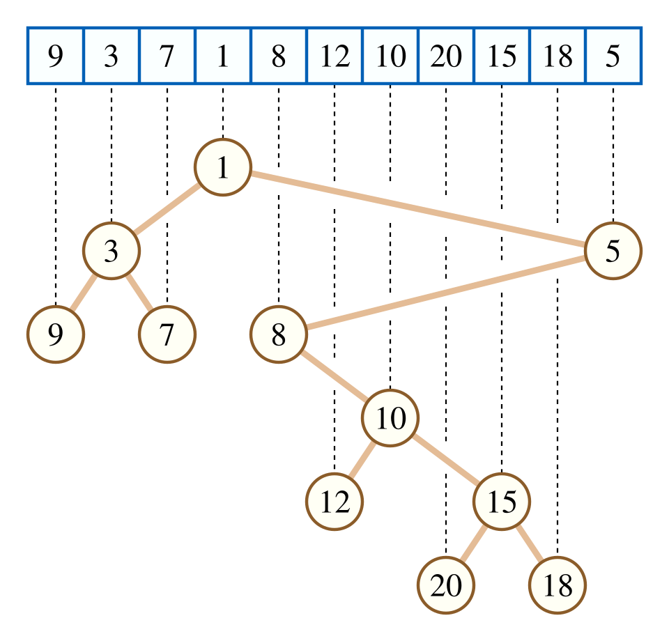
We can use \(\rmq(1,n)=i\) to find the smallest element in the array. Then, we can use \(\rmq(1, i-1)\) to find the smallest element left of it (if \(i>1\)) and \(\rmq(i+1, n)\) to find the smallest element right of it (if \(i < n\)).
Cartesian trees. The Cartesian tree is the binary tree we get by repeating this process recursively, where nodes are numbered in-order from left to right. Specifically, the Cartesian tree fully encodes the \(\rmq\) answers: \(\rmq(i,j)\) is (the label of) the lowest common answer of nodes \(i\) and \(j\).
This also implies that any two different trees correspond to different \(\rmq\) answers: given two distinct trees, compare them recursively starting at the root. As soon as a node has a different label in the two trees, that means the \(\rmq\) of the interval of the corresponding subtrees differs in the two cases.
Thus, the \(\rmq\) answers are in bijection with Cartesian trees, and the number of bits we need to encode all \(\rmq\) values is the log of the number of Cartesian trees.
Binary trees. Cartesian trees are simply binary trees wit an in-order numbering of the nodes. Binary trees are in bijection with the ordered rooted trees we saw before (wikipedia):
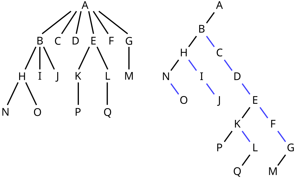
In the binary tree, each edge to the left introduces a child, while each edge to the right means the two nodes are siblings.
As we already saw before, the number of ordered trees on \(n\) nodes is the Catalan number \[ C_n := \frac 1{n+1} \binom{2n}n \sim \frac{4^n}{n^{3/2}\sqrt \pi}. \] Thus, the number of Cartesian trees is the same and the number of bits needed to represent one is \[\log_2 C_n = 2n - \Theta(n).\]
So the goal is: RMQ with \(2n\) bits and constant-time queries.
As an aside, Fischer and Heun (2011) show that if we have access to \(A\), we can trade space for query time and have \(2n/c(n)\) bits of space with query-time \(O(c(n))\). Basically, we can split \(A\) in blocks of size \(c(n)\), build the RMQ data structure on the \(n/c(n)\) blocks in \(2n/c(n)\) bits, and then use \(A\) to find the minimum of each block in \(c(n)\) time.
3 Sparse Table: \(O(1)\) queries, \(O(n \log_2 n)\) words Link to heading
Let \(k = \lfloor \log_2 n \rfloor\).
Store a tree of \(k+1\) levels \(0, \dots, k\).
In level \(\ell\), store \(n+1-2^\ell\) values for \(0\leq i < n+1-2^\ell\), each storing the minimum over a (sliding) window of length \(2^\ell\): \[S_\ell[i] := \min_{i\leq j < i + 2^\ell} a_i.\]
To answer a query \([l,r)\), first find the largest power \(2^\ell\) that is at most \(r-l\). Then we have \[l \leq r-2^\ell \leq l + 2^\ell \leq r,\] i.e., the intervals \([l, l+2^\ell)\) and \([r-2^\ell, r)\) together cover \([l, r)\). Thus, we get: \[\min_{l\leq i< r} a_i = \min(S_\ell[l], S_\ell[r-2^\ell]).\]
To get the index of the minimum, store that instead, and take the argmin over the two indices returned by the two lookups.
4 Segment Tree: \(O(\log n)\) queries, \(O(n)\) words Link to heading
Sparse tables are quire redundant since consecutive nodes store mostly the same information. Segment trees reduce the space usage, but have slower query times.
- Again, use \(k=\lfloor \log_2 n\rfloor\) and make levels \(\ell\in\{0, 1, \dots, k\}\).
- Level \(\ell\) has \(\lfloor n/2^\ell\rfloor\) nodes, each storing the minimum over a chunk of length \(2^\ell\): \[S_\ell[i] := \min_{i\cdot 2^\ell \leq j < (i + 1)\cdot 2^\ell} a_j.\]
- To query an interval \([l, r)\), we check for each level whether to include a
segment from that level or not.
- If \(l\) is odd, use \(S_0[l]\) and then increment \(l\) by \(1\).
- If \(r\) is odd, use \(S_0[r-1]\) and then decrement \(r\) by \(1\).
- Then:
- if \(l\bmod 4 = 2\), use \(S_1[l/2]\) and increment \(l\) by \(2\).
- if \(r\bmod 4 = 2\), use \(S_1[r/2-1]\) and decrement \(r\) by \(2\).
- Then:
- if \(l\bmod 8 = 4\), use \(S_2[l/4]\) and increment \(l\) by \(4\).
- if \(r\bmod 8 = 4\), use \(S_2[r/4-1]\) and decrement \(r\) by \(4\).
- Continue this with increasing powers of \(2\), until \(l=r\).
In practice, the segment tree admits a nice linear data layout where the data of all levels is concatenated.
5 Blocks: \(O(s)\) queries, \(O(n/s \log n)\) words Link to heading
A technique we’ve seen before with rank & select is to use a simple but space-consuming technique on a sufficiently sparse subset of the data. Here we can do the same:
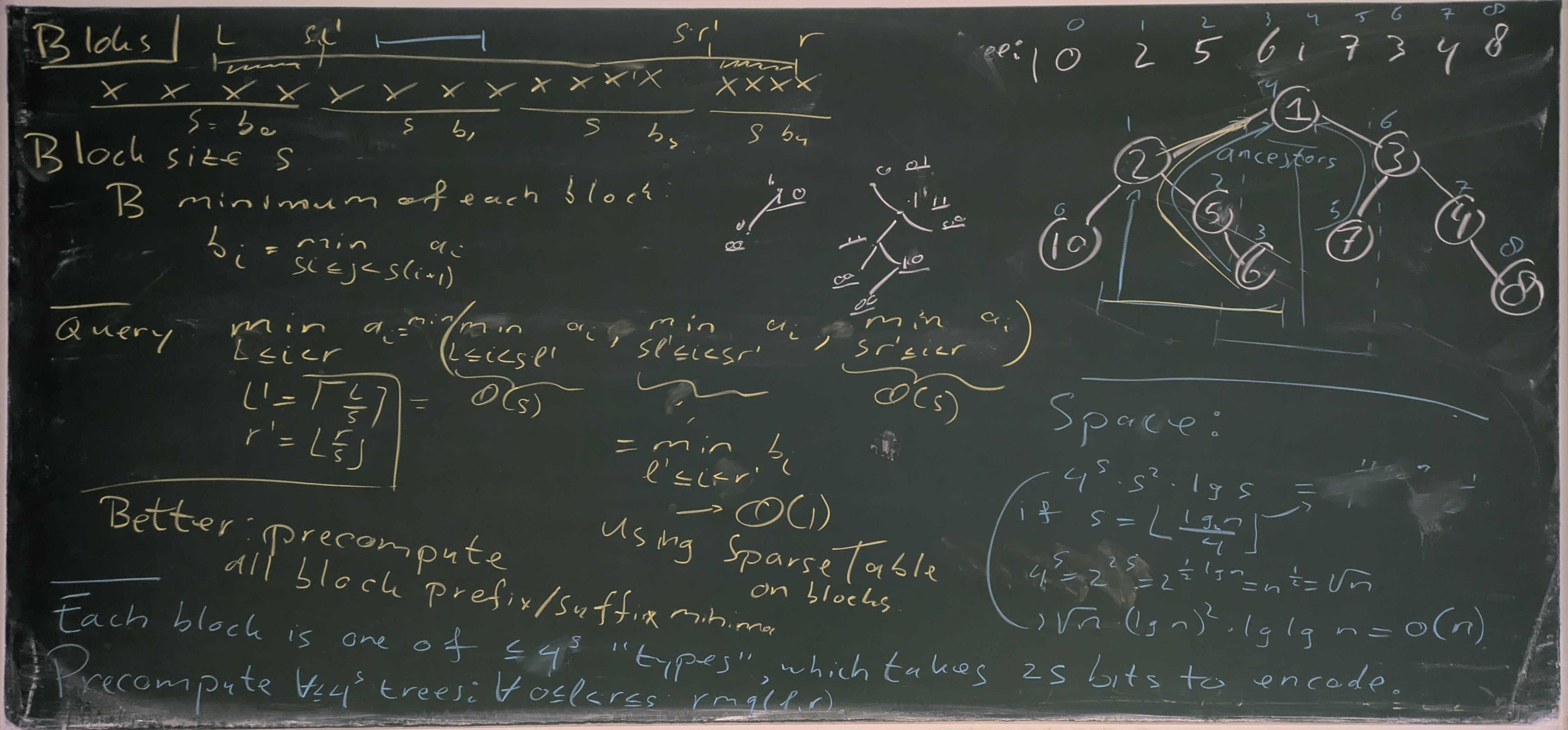
- Split the data into \(n/s\) blocks of size \(s\): \[b_i := \min_{i\cdot s \leq j < (i+1)\cdot s} a_i.\]
- Store a sparse table over the \(b_i\), consuming \(O(n/s \cdot \log(n/s)) \leq O(n/s \log n)\) words.
- To answer a query \([l, r)\), compute \(l’=\lceil l/s\rceil\) and \(r’=\lfloor r/s\rfloor\). Then return \[\min_{l\leq i < r}a_i = \min_{l\leq i < l’\cdot s} a_i + \min_{l’\leq i’ < r’} b_{i’} + \min_{r’\cdot s\leq i < r} a_i.\]
- This takes \(O(s)\) for computing the minimum of the suffix of the first block and the minimum of the prefix of the last block, and \(O(1)\) for the sparse-table lookups for the middle.
- If \(s=\log_2 n\), this gives (like the segment tree) \(O(\log n)\) queries and \(O(n)\) memory.
- Storing the suffix and prefix minima of each block takes \(2n\) words, which fits in the \(O(n)\) budget. That makes most queries \(O(1)\), apart from those where \([l, r)\) is contained entirely within a single block.
6 Cartesian Trees: \(O(1)\) queries, \(O(n)\) words Link to heading
Cartesian trees can be used to efficiently answer the within-block queries.
As we saw before, there are \(o(4^s)\) possible Cartesian trees (and thus sets of possible answers) for a block of size \(s\).
Choosing \(s=\frac 12 \log_4 n = \frac 14 \log_2 n\), there are \(\sqrt n\) different cartesian trees.
We can now do the same trick as we saw before for popcount:
- there are \(4^s = o(\sqrt n)\) trees;
- for each, there are \(\binom{s+1}2 = O(s^2) = O(\log^2 n)\) possible queries;
- the position of the minimum takes \(\log_2 s = O(\log \log n)\) bits to store
for a total precomputation space of \[4^s s^2 \log_2 s = O(\sqrt n \cdot \log^2 n \cdot \log\log n) = o(n).\]
All that remains is to store for each block its “shape” (see below): a \(2s\)-bit string encoding its Cartesian tree. When storing these in a “bitpacked vector”, this takes a total of \(2s \cdot n/s = 2n\) bits, exactly matching the lower bound!
When used in combination with the block-based sparse table above, we can also use the Cartesian trees for the precomputed index of the prefix/suffix minimum.
Encoding Cartesian Trees. As we saw before, the number of Cartesian trees on \(n\) nodes is the Catalan number \(C_n = \frac 1{n+1}\binom {2n} n \leq 2^{2(s-1)}\). Thus, \(2(s-1)\) bits suffice to encode it, but here we will use \(2s\) instead.
We already saw that Cartesian trees are simply (non-balanced!) binary trees. Binary trees can be encoded in many ways:
by using the bijection to ordered trees and using a method from last lecture (LOUDS/DFUDS/BS).
by extending the tree with leaves so that all original nodes have degree 2, and then traversing the tree in BFS or DFS order, writing 1 for each internal node and 0 for each leaf.
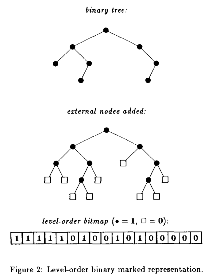
Figure 1: Figure from Jacobson (1989)
Or maybe simplest: by writing for each node whether it has a left child (1 or 0) and whether it has a right child (1 or 0) and then traversing the tree in DFS or BFS order.
Overview. All-together, we store:
- precomputed query answers for all Cartesian trees in \(o(n)\) bits total;
- for each block, its Cartesian tree in \(2n\) bits total;
- the sparse table on block-minima, in \(O(n/s \cdot \log n) = O(n)\) words.
Thus, the sparse table is the largest part.
7 Recursive Cartesian Trees: \(O(1)\) queries, \(2n+o(n)\) bits Link to heading
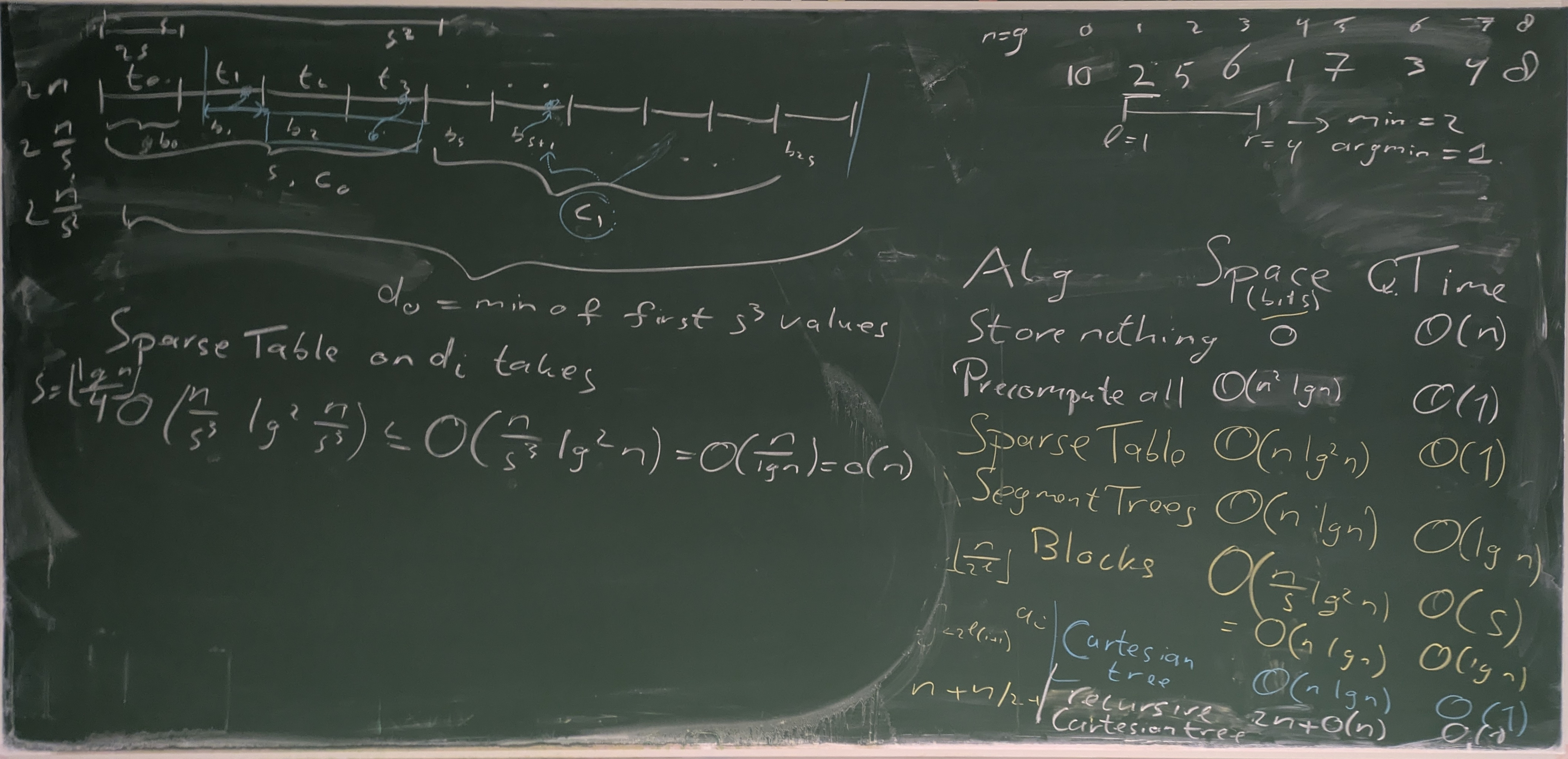
To reduce the space from \(O(n)\) words, we need to make the blocks larger so that the sparse table is smaller. To this effect, we can use the Cartesian tree technique recursively on the block-minima \(b_i\) (see section 3.3 of Fischer and Heun (2011)), but repeated recursion would not give constant queries.
Applying the recursion once, that is, effectively using a sparse table on blocks of size \(s^2\), makes it use \(O(n/s^2 \log(n/s^2)) \leq O(n / \log^2 n \log n) = O(n /\log n)\) words of space, or \(O(n)\) bits.
Using the recursion one more time, for a total of three layers of Cartesian trees, yields \(O(n/s^3 \log(n/s^3)) \leq O(n/\log^3 n \log n) = O(n/\log^2 n)\) words, or \(O(n / \log n) = o(n)\) bits of space, for \(2n + o(n)\) bits of space all together! Most bits are used to store the type of the Cartesian trees at the root level.
One thing to note is that ‘unpacking’ the answer requires multiple steps now: if the recursive tree gives a minimum in block \(b_i\), then we must get the type of that block and do a lookup to find the position of the minimum inside the block.
8 Blackboard Link to heading