Models of computation
Advanced Data Structures – Summer 2026 – Lecture 1
Ragnar {Groot Koerkamp}, Stefan Walzer, Stefan Hermann
2026-04-20 Mon 14:00
curiouscoding.nl/teaching
Today
- Why do we care about models?
- Big-\(O\) notation
- The complexity of sorting
- Properties data structures
- The word RAM model
- Variations
- Limitations
Motivation
Motivation
We want to design fast algorithms, but when is an algorithm fast?
- Implement it, and measure the time.
- Extrapolate experiments to predict performance on larger \(n\).
- May or may not give understanding.
- Does not provide lower bounds.
- Analyse exactly what happens on the CPU.
- Unwieldy; they are massive black boxes.
- Instead: use a simplified abstract model of the CPU.
- Allows exact lower and upper bounds.
Big-O notation (recap)
Big-O notation (recap)
Big-\(O\), or \(\mathcal O\) notation relates the asymptotic growth of two abstract functions to each other.
Given two functions \(f, g: \mathbb N \to \mathbb R_{\geq 0}\), we say that
when there exists constants \(n_0\in \mathbb N\) and \(M\in \mathbb R\) such that for all sufficiently large \(n\geq n_0\): \[ f(n) \leq M\cdot g(n).\]
- \(f(n) = o(g(n))\) is like \(<\): \[\lim_{n\to\infty} f(n)/g(n) \to 0.\]
- \(f(n) = O(g(n))\) is like \(\leq\): \[f(n) \leq M\cdot g(n) \quad \forall n\geq n_0.\]
- \(f(n) = \Theta(g(n))\) is like \(=\): \[f(n) = O(g(n)) \text{ and } g(n) = O(f(n)).\]
- \(f(n) \sim g(n)\) is a stronger \(\Theta\): \[\lim_{n\to\infty} f(n)/g(n) = 1.\]
- \(f(n) = \Omega(g(n))\) is like \(\geq\): \[f(n) \geq M\cdot g(n) \quad \forall n\geq n_0.\]
- \(f(n) = \omega(g(n))\) is like \(>\): \[\limsup_{n\to\infty} f(n)/g(n) \to \infty.\]
Quiz time!
What is the complexity of sorting?
What is the complexity of sorting?
- \(O(n \lg n)\)?
- \(O(n \lg w)\)?
- \(O(n \sqrt {\lg n})\)?
- \(O(n \sqrt {\lg \lg n})\)?
- Linear \(O(n)\)?
- Constant \(O(1)\)?
- Something else?
What is the complexity of sorting?
All of the above!
- \(O(n \lg n)\)
- Minimum number of comparisons is \(\Omega(n \lg n)\).
- Merge sort indeed uses \(O(n \lg n)\) of them.
- Or QuickSort, with \(O(n \lg n)\) comparisons in expectation.
- \(O(n \lg w)\)
Expected complexity of Van Emde-Boas trees
- \(O(n \sqrt {\lg n})\)
- Fusion trees (Fredman and Willard 1993)
- \(O(n \sqrt {\lg \lg n})\), \(O(n\sqrt{\lg w})\)
Fastest randomized algorithm
- Linear \(O(n)\)
- Linear space? Sure!
- Counting sort when all values are \(O(n)\).
- Radix sort on 64-bit integers.
Randomized when \(w \geq (\lg n)^{2+\varepsilon}\)
- Constant \(O(1)\)
- \(n \leq 2^{64}\) makes \(f(n)\) bounded.
- There's only so many atoms in the universe.
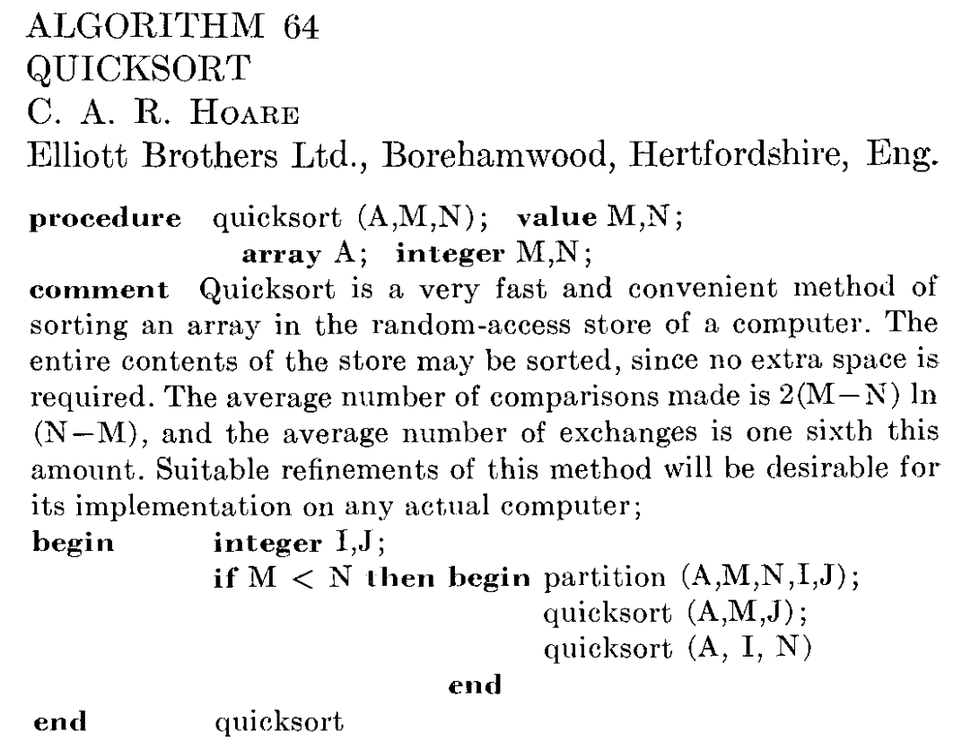
Figure 1: Algorithm 64: Quicksort (Hoare 1961). RIP Tony Hoare.
"Complexity"
"Complexity"
- Lower or upper bound?
- Complexity of a problem is at least \(\Omega(\dots)\).
- Complexity of an algorithm at most \(O(\dots)\).
- "The complexity": matching lower and upper bound.
- Which metric?
- "Operations"
- Comparisons
- Memory accesses
- Memory touched
- Wall time
- Space usage
- What input type?
- Integers
- Floats
- Abstract "objects"
- What input properties?
- (Uniform?) random
- Worst-case
- What algorithmic properties?
- Deterministic
- Randomized
Properties of data structures
Space usage
Let \(S\) be the minimum space required to represent some data.
A compact data structure uses \(O(S)\) bits of space.
A succinct data structure uses \(S + o(S)\) bits of space.
Example: many Rank & Select data structures are succinct.
An implicit data structure uses \(S + O(1)\) bits of space.
Example: bit arrays.
Dynamic data structures
Allows mutating the structure.
Example: hash tables.
Build once, then read-only queries.
Example: minimal perfect hash functions.
Insert-only; deletions not allowed.
Example: bloom filters.
Running time
From stronger to weaker:
An algorithm has worst-case running time \(O(f(n))\) when for every possible input, it is guaranteed to finishes in \(O(f(n))\) time.
An algorithm has expected running time \(O(f(n))\) when for every possible input, the expected running time is \(O(f(n))\).
An algorithm has running time \(O(f(n))\) with high probability (w.h.p.) when for every possible input, the running time is \(O(f(n))\) with probability \(1-o(1)\).
Running time
An operation on a data structure has amortized running time \(O(f(n))\) when for every possible sequence of \(i\) operations with amortized complexities \(f_i\), the total running time is \(O(\sum_i f_i)\).
Example: pushing on a vector is worst-case \(O(n)\), but amortized \(O(1)\).
Models of computation
The RAM model
Models a machine that has an infinite list of registers.
- Each register can store an unbounded (!) natural number!
- Each register has an address.
- Retrieving the register corresponding to an address takes constant time.
Any problems with this?
The real RAM model
Like the RAM model, but each register can store a real number.
The word RAM model
Like the RAM model, but operates on words of \(w\) bits.
- Registers are also \(w\) bits.
- Constant-time \(w\)-bit arithmetic operations:
- bit-operations, addition, multiplication.
Evolved with CPUs to include: https://en.wikipedia.org/wiki/X86_Bit_manipulation_instruction_set
- Popcount (
popcnt), count trailing zeros (tzcnt, BMI1) - Parallel bit deposit (
pdep), parallel bit extract (pext, BMI2)
Most commonly used model.
Any remaining problems with this?
We must talk about \(w\)
We must talk about \(w\)
- In practice, \(w=64\) is constant.
- But the problem size \(n\) grows to infinity.
- What if \(n > 2^w\)? Then we can't even represent \(n\)?
Solution: we assume \[ \lg n \leq w. \] This has far-reaching implications!
- The complexity of pop-counting \(n\) bits is sub-linear \(O(n / \lg n)\)!
- Fusion trees can binary search on \(O(\sqrt w)\) \(w\)-bit integers in constant \(O(1)\) time!
The pointer model
RAM-model without the RAM:
- Registers can only be accessed via direct pointers.
Used in the analysis of some heap-based priority queues.
The cell-probe model
Like the RAM-model, but all operations apart from accessing memory are free.
- Typically, an infinite cache is assumed, so that each address only has to be read once.
- Used for lower bounds on the number of addresses that must be read to solve some task, and thus a lower bound on RAM-model complexity.
The RAM-model is unphysical
The RAM-model is unphysical
- Infinite memory with constant time access is fundamentally not possible:
- Each bit takes some small volume \(v\) to store.
- Signals can only travel at the speed of light \(c\).
- In time \(t\), we can read from a sphere of radius \(tc\), containing \[\frac 43 \pi (tc)^3/v = \Theta(t^3)\quad \text{ bits}.\]
The latency of a uniform random access into a memory of size \(n\) is at least \[\Omega(\sqrt[3]{n}).\]
The RAM-model is unphysical (2)
The RAM-model is unphysical (2)
- Black holes have only quadratic mass \(\Theta(r^2)\)!
- Filling a volume with cubic information is impossible.
- But we are far away from the constant.
- If each bit of memory requires some energy, we need to dissipate \(\Theta(r^3)\)
heat through \(\Theta(r^2)\) of surface area.
- This is an actual bottleneck for CPUs! They are mostly flat (2.5D) for a reason!
- AMD now has "3D V-Cache" which vertically stacks caches.
- This is an actual bottleneck for CPUs! They are mostly flat (2.5D) for a reason!
We can store/cool at most \(O(r^2)\) bits in a sphere of radius \(r\), and so the latency of a uniform random access into a memory of size \(n\) is at least \[\Omega(\sqrt[2]{n}).\]
- See this blog: The Myth of RAM
The RAM-model is unrealistic

- Green: latency of array indexing.
- Clearly not \(O(1)\)!
- More like \(\sqrt[3] n\) (dashed blue)
- Black: latency of binary search.
- Clearly not \(O(\lg n)\) (solid blue)
- Red: binary search with heap-layout
- \(<3\times\) slower than just indexing?!
\(\sqrt[3]{1} + \sqrt[3]{2}+\dots+\sqrt[3]{n} = \Theta(\sqrt[3]n)\).
- TODO: \(\sqrt n\)-complexity model!
The I/O-complexity
Introduced by Aggarwal and Vitter (1988).
Like the cell-probe model, the I/O-complexity only counts I/O operations.
- Fast and free internal memory of \(M\) words.
- Slow (infinite) external memory.
- Count I/O-operations between them go in blocks of \(B\) words.
Sorting \(n\) word-sized integers has an I/O-complexity lower-bound of \[ \Omega\left(\frac n B \log_{M/B} \frac nB\right), \] and external merge-sort achieves this.
Takeaways
We need precisely defined models to theoretically analyse algorithms.
Models approximate reality; some do so better than others.
The rest of this course will mostly use the word RAM model to analyse both theoretically and practically efficient algorithms.
Further reading
- These slides: curiouscoding.nl/teaching
- Algorithmica on binary search:
- https://en.algorithmica.org/hpc/data-structures/binary-search/
- Great resource for understanding and optimizing for modern CPUs
- Paper: Array layouts for comparison-based searching (Khuong and Morin 2017)
- Blog: The Myth of RAM
- My P99 talk on binary search
- Aggarwal and Vitter's slides on I/O-complexity:
Next week: Bitvectors, Rank, & Select
Bibliography
Possible exam questions
- What is big-O notation? Name some of the different variants.
- What are some problems with saying "the complexity of sorting"?
- Give an example of a precisely specified complexity of an algorithm.
- What is the difference between compact, succinct, and implicit data structures? Give an example for each of them.
- What is the difference between worst-case, expected, and amortized running time?
- Name 5 different models of computation.
- What are some problems with the word RAM model? Why do we use it anyway? Is there a model that solves these issues?
- What can you say about \(w\)?